Messi or Ronaldo? Kroos or Modric? Mbappe or Neymar? Every football fan loves to argue over who they think is a better player. Depending on where your loyalties lie, arguments can range from simple statistics; like the number of goals they’ve scored or the trophies they have won, to advanced metrics like expected goal values from ghosting. To the layman football fan, the former argument is almost certainly more digestible. But for the rest of us, we often want a metric that’s more objective, more extendable, and more rigorous, while still being able to understand it and explain it to your counterpart to assert your football dominance.
The evolution of football analytics - how we got to non-shot expected goals models.
Every football analytics nerd understands the (slow) evolution of football statistics. The story begins with football’s notorious and frustratingly difficult objective of scoring goals, the historic hindrance for American spectating. Analyzing goals scored and goals conceded appeased few and people quickly realized the value of shot volume for depicting a team’s performance and ability. The obvious pitfall in comparing shot volume was the quality of a shot can vary drastically. This led to everyone under the sun defining their own expected goals (xG) model to objectify chance quality and aggregate goal likelihood as a better metric for attacking production. xG is now omnipresent in football analytics as a tool for attackers’ and teams’ performance. Most recently in the sports analytics community, people have extended the concept of expected goals to allocate ball progression contributions throughout a team’s possession of the ball.
Commonly referred to as “non-shot expected goals (NSxG) models”, these models are effective tools to quantify passes and carries into dangerous areas of the pitch, assigning value to actions other than shots and allowing for the comparison of attacking contribution of ALL players. Fivethirtyeight even uses a non-shot xG model as a component in their soccer projections.
The original research - before “non-shot expected goals” became a thing - was by Sarah Rudd, presented at NESSIS in 2011. Rudd used markov models to assign individuals offensive production values defined as the change in the probability of a possession ending in a goal from the previous state of possession to the current state of possession.
For example, imagine a player standing 30 yards from the goal line, close to the sideline. They are in a non-threatening position and that possession will rarely result in a goal. Let’s say it has a 1% chance of resulting in a goal. Now, that player gets a cross off, the defender clears it out of bounds for a corner kick. Corner kicks resulted in goals approximately 4% of the time. This play would attribute a +3% change in NSxG for the player who crossed the ball.
As data becomes increasingly utilized and accessible, the variants of NSxG models grow just as xG models did. Mark Taylor further explains NSxG models here. Nils Mackay defines “xG added” to grade passing skill and extends it to allocate value for carries and structures as a possession based model. Similarly (and most recently), Karun Singh published his version of xG added, introducing xG threat, explaining it with beautiful interactive visualizations.
All of this publicly facing research has been pivotal in advancing the applications and effectiveness of sports analytics. Today, I am going to walk through a tutorial on StatsBomb’s first iteration of a Ball Progression Model. I like to refer to NSxG as “contribution”, simply because it's easier to say and not everything in football analytics needs an “x” in it.
Markov Model - Framework and Methodology.
Adopting the framework set forth by Rudd, we construct a possession based markov model we call our “Ball Progression Model”. We define attacking possessions to have two possible outcomes, a Goal or a Turnover. In a markov model, these two outcomes are known as the “absorption states”. The most crucial condition of an absorption state is that the probability of transitioning out of the state is 0 and the probability of remaining in the state is 1, given that it is the end of a possession this condition holds and the data must be structured as such (this condition makes it more difficult to consider shots or xG bins as potential absorption states). Leading up to the absorption state, a possession can transition between any number of “transient states”. We define transient states based on the context of the state and the geographical location of the possession at a current state. Extending the states defined by Rudd and applying to StatsBomb data, we define the following context-based transient states:
- Attacking Third Free Kick
- Central Third Free Kick
- Defending Third Free Kick
- Attacking Third Throw In
- Central Third Throw In
- Defending Third Throw In
- Corner Kick
- Penalty Won
We then define the following geographic zones as transient states:
![]() Since a state can depend greatly on defensive pressure, we define the geographic zones each when they are absent of pressure and when they are under pressure. This leaves us with 76 geographic zones (38 with pressure, 38 without pressure) and 8 contextual zones for a total of 84 transient states.
Since a state can depend greatly on defensive pressure, we define the geographic zones each when they are absent of pressure and when they are under pressure. This leaves us with 76 geographic zones (38 with pressure, 38 without pressure) and 8 contextual zones for a total of 84 transient states.
Transient states can transition between other transient states and ultimately an absorption state based on some observed transition probability. The transition probability is dependent only on the current state of the possession and is independent of previous states. This is known as the markov property and is a key assumption in markov models (in the discussion we consider this a limitation and propose extensions to this property). For instance, if you have the ball in zone 21, the probability that you pass the ball to zone 28 is the same regardless of the fact that the ball came from zone 14 as opposed to any other zone. This is known as the “memoryless” property.
Quick notation - n is the number of transient states (in our case 84), r is the number of absorbing states (in our case 2). Q is the matrix of transition probabilities, Q is n x n. R is the matrix of absorption probabilities, R is n x r. N is known as the fundamental matrix and it is calculated as the inverse to the n x n identity matrix, I, minus the transition matrix Q, formally N = (I - Q)-1 .
Calculations - for each transient state, we can calculate the expected number of plays (progressing actions: passes, carries, and shots) until absorption as the row sums of the fundamental matrix. Then, the probability of reaching either absorption state for the current transient state is equal to N x R. For more on the theory behind markov models, please see here. Special thanks to Ron Yurko for the code.
Results
We prepare the data (this is the most time consuming portion) and run our ball progression model for Europe’s big five leagues, England Championship and England League One for the 2017/2018 and 2018/2019 (through 2/18/19) seasons.
For each transient state, we calculate the probability of a goal in absorption as well as the expected number of plays until absorption. The three most likely states to result in a goal are (refer to geographic zones above): 36 w/ pressure (Pr(Goal) = 19.2%), 31 w/ pressure (Pr(Goal) = 9%), and 36 w/o pressure (Pr(Goal) = 8.3%). The three most likely zones to result in a turnover are: 1 w/ pressure (Pr(Turnover) = 99.5%), 3 w/ pressure (Pr(Turnover) = 99.5%), and 2 w/ pressure (Pr(Turnover) = 99.5%). We present a possession that resulted in a goal below, with the contribution value for each action.
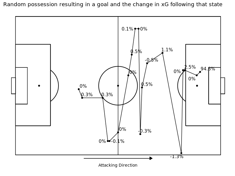 We then calculate our “contribution” metric as the change in the probability of a goal from the current state to the next state. Formally,
contribution = Pr(Goal|Statet+1) - Pr(Goal|Statet) for each transient state at time t.
We can also calculate total attacking contributions for each individual, i, as the sum of all of their attacking contributions,
contributioni = ∑Pr(Goal|Statet+1) - Pr(Goal|Statet)i ·I(action by player i)
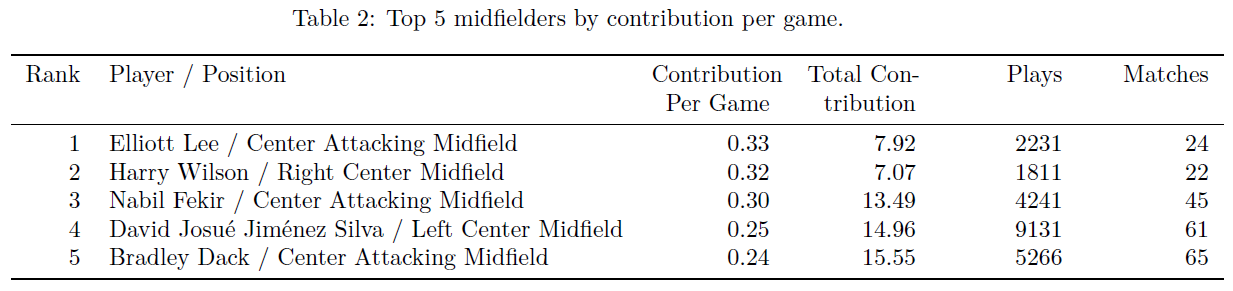
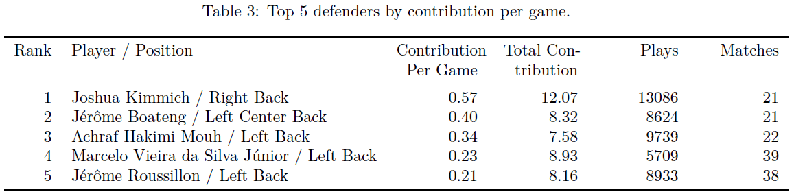
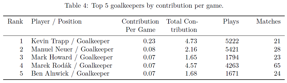
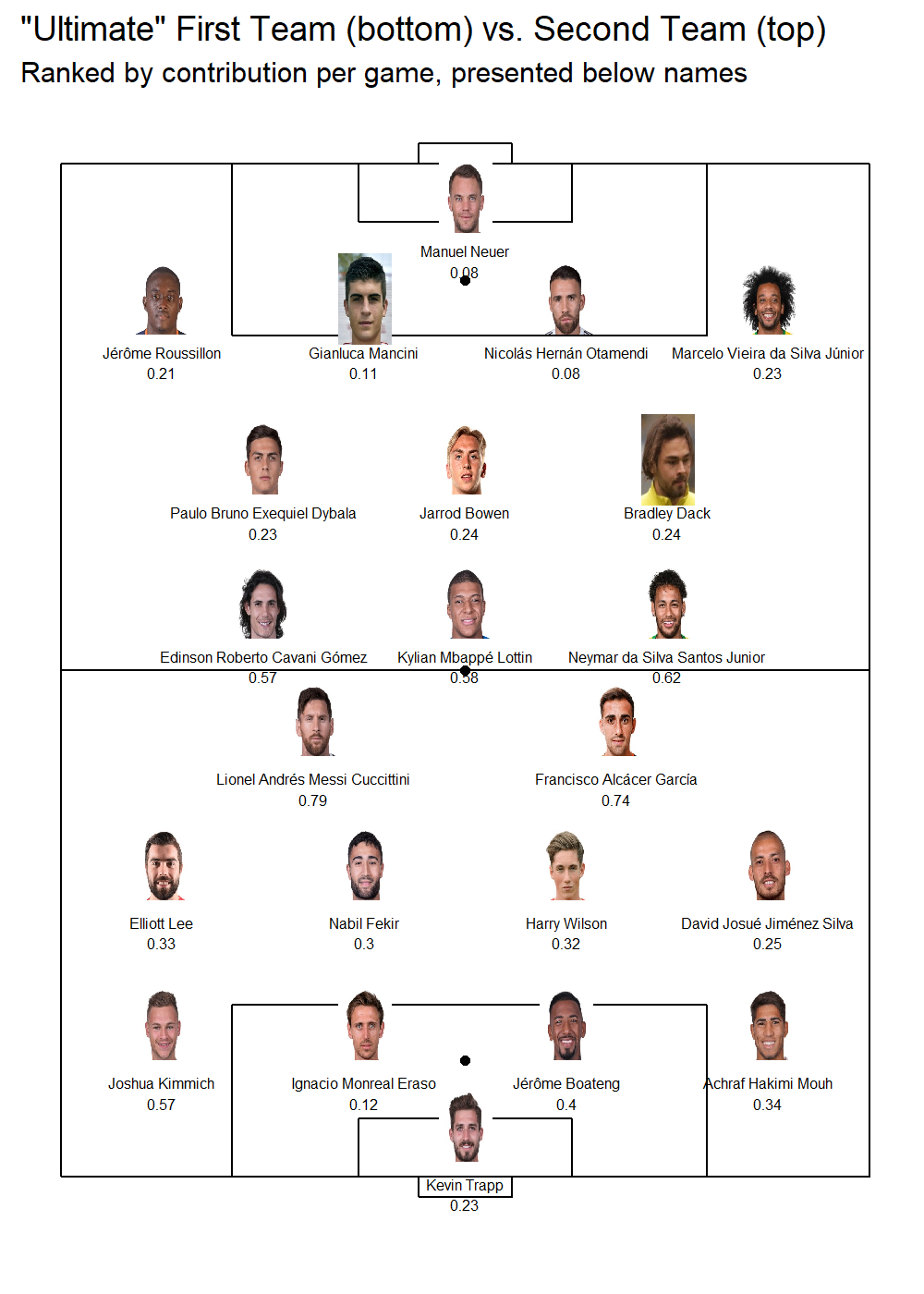
We then scale their total contribution by the number of matches played to get a player’s “contribution per game”. We choose to leave the contribution per game metric raw, not standardizing by league strength. This is to simply to see the crude output from the model, giving every player a fair chance to shine regardless of where they play. The top five contributors for each position (attackers, midfielders, defenders and goalkeepers) are presented in the tables below:
We also formulate a hypothetical “Ultimate Team” for the top contributors for each position of a standard 4-4-2 against a 4-3-3. Again, we purposely make the naive assumption that contributions between different leagues are equal. We also, in order to show you some names you might know, purposely didn't stress that the ultimate teams are extremely broad and unrealistic when it comes to positional categorizations. The two squads we formulate highlight plenty of young stars to remember during the next transfer window.
 Discussion
Our ball progression model has clearly identified the top players across Europe, and offers some justification for the money needed to acquire them. We have clearly designed a model that is easily interpretable even by the less-technical analytics sides. And ultimately, the model works without much computational power. Markov models are good at handling sequences of arbitrary length (as possessions in soccer can be anywhere from one event to 100s of events), and they allow for the attribution of final outcome contributions further along in the sequence. Nonetheless, there exist several limitations to a simple markov model.
- First, markov models’ assume the “memoryless” property when in reality a soccer possession is not memoryless. The probability of scoring when you are in a current state can depend on previous passes and carries leading up to the current state.
- A further extension of our ball progression model, that would appease this limitation, is higher order markov models. In higher order markov models, instead of assuming the markov property of independence, you assume that transition probabilities are conditionally independent based on the value of the current state and the value of the previous, 2nd previous, nth previous state, where the number of previous states you consider is the nth order of the markov model.
- Another limitation is that this simple markov model does not consider the action required to transition between states. For instance, the probability of a possession resulting in a goal may be different given that you passed into a zone vs. dribbled into a zone.
- Lastly, and perhaps the most obvious limitation of this markov model is the categorized structure of transient and absorption states. This causes the loss of information and limits applications especially in the free-flowing game of football.
- There exists some methods for continuous stochastic processes, but their use in the public sphere is limited and the concepts are far more difficult to understand.
This leads us to StatsBomb’s latest endeavor. Based on the limitations outlined above, we recognized the need for a model that accounts for the continuous nature of football, the retention of information from previous states, and the actions chosen by decision makers. Our next model will improve on the limitations noted above as well as layer on additional components essential to a football team’s success such as the timing of goals and the style of play under different game states. This will be the primary model we use for holistic ball progression in player and team stats, and a white paper detailing the model will be made available to current StatsBomb customers in March.