First, a disclaimer: the use of the following player examples to demonstrate a bit of statistical theory is by no means a criticism or an opinion on their footballing ability. Oh, and I’m actually a Liverpool supporter so this is definitely NOT a dig at Suarez! Now that the disclaimer is out of the way let’s start: Luis Suarez has so far scored 23 goals in 19 league appearances. Sergio Aguero has scored 15 goals in 15 starting and 2 substitute appearances. Let’s call them a total of 17 appearances for now and we can deal with this later on. Here are these figures in summary:  Based on these numbers Suarez is scoring at a much higher rate than Aguero. But could this simply be randomness instead of anything else? It’s time for a bit of statistics. Goals, shots, tackles, interceptions and lots of other match statistics can be thought of as random variables, which follow a probability distribution. So if you were to collect a zillion matches, a p0 percentage of them would have 0 events occurring (e.g. goals) , p1 would have exactly 1 event occurring, p2 would have exactly 2 events and …. Well, you get the drift. These probabilities (p0, p1, p2, …) form the probability distribution. One distribution that is often used when dealing with the occurrence of events is the Poisson distribution. Given a mean, it tells us the probability of an event happening 0, 1, 2, 3, … times within a particular period. So for example, with an average rate of 1.21 goals per match, Suarez has the following goal probability distribution in a match:
 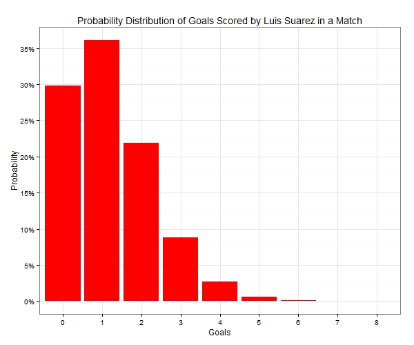 There is about 30% of him not scoring in a randomly selected match, around 36% of scoring exactly once and almost 9% of scoring a hat-trick (actually exactly 3 goals and not more!). Furthermore, if we were to look at the number of goals Suarez was likely to score in 19 matches, again using the average rate of 1.21 goals per match, the probability distribution would now look like the following:
 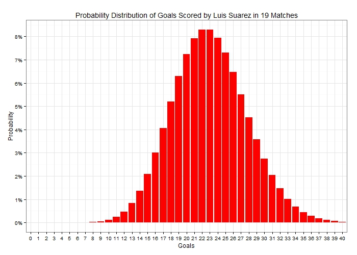 Notice how the probability distribution approaches the bell-shaped Normal distribution as the sample size i.e. the number of matches increases. This is a result of what is known in statistics as the Central Limit Theorem. A very important takeaway from the above graph is that there is a lot of uncertainty in the actual number of goals scored. In fact scoring exactly 23 goals in 19 appearances – as he has done so far in the Premier League – has a probability of just 8.3%. So let’s now turn our attention to Sergio Aguero, too. He scores at an average rate of 0.88 goals per match so if we were to add his goal probability distribution for a single match next to Suarez’s it would look like this:
 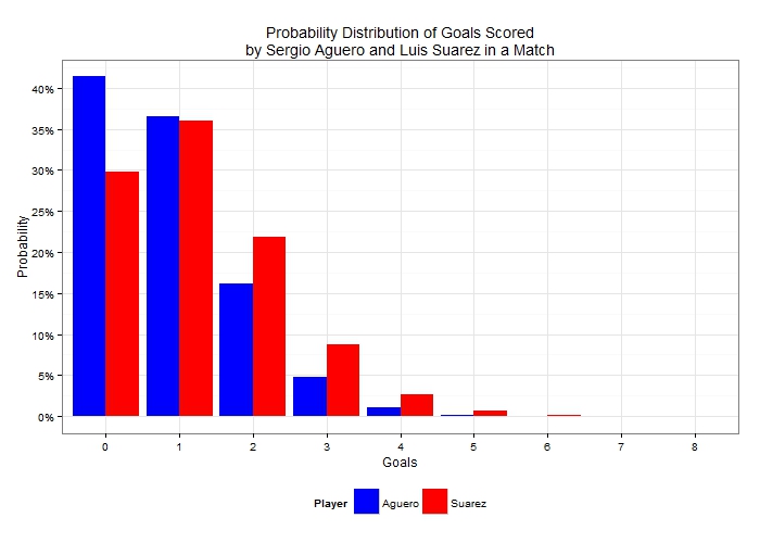 Since Aguero has a lower scoring rate, his probability mass is shifted towards the lower number of goals compared to Suarez’s. He has more than 41% chance of ending the match without a goal and less than 5% chance of getting exactly 3 goals. Looking at these players over a wider sample, it would be unfair to compare the distribution of goals in Aguero’s 17 appearances with Suarez’s 19 appearances so let’s see how those two distributions would look like (given their respective average scoring rates per match) if both had played 19 matches:
 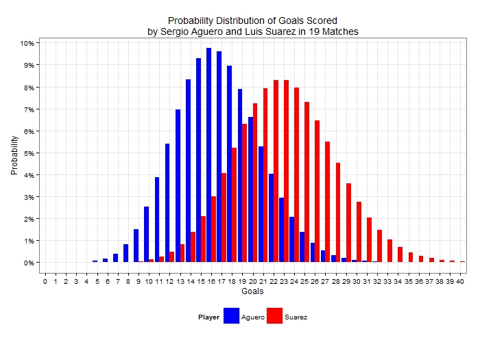 Evidently even though Suarez is generally expected to score a higher number of goals in those 19 matches, it is possible for Aguero to outscore him. It’s therefore important, before jumping into any conclusions about the relative levels of scoring ability between the two players to take into consideration this uncertainty that is demonstrated by the two distributions. To compare these scoring records we can use statistical significance tests which allow us to decide whether there is significant difference between scoring rates or whether any observed differences could simply be attributed to randomness. To carry out a significance test, a null hypothesis is first formulated. In this example, the null hypothesis is that of no difference between the scoring rates of the two players. Then test-statistics are calculated, which in turn result in what is known as a “p-value”. To cut a long story short, and to spare the few readers still following me the statistical theory behind this, we can compare the p-value with small probabilities (usually 5% or 1% which are the chosen significance levels). If the p-value is a very small number – smaller than the significance level – then there is evidence in the data that leads us to reject the null hypothesis. If the p-value is large then the statistical test has failed to reject the null hypothesis, or in this particular case that the two scoring rates could in fact be equal and any observed difference is simply down to randomness. Interestingly enough, comparing Poisson means is not as widespread as means of other distributions but a widely used test is the conditional test developed by Przyborowski and Wilenski (1940). As I don’t want you to be scared away from the maths expression, I’ll jump straight to the p-value result! (But for those of you interested you can scroll at the end for the algebraic expression and then back to continue.) Applying the conditional test to the data at the start of the article (23 goals in 19 matches against 15 goals in 17 matches) results in a p-value of ……. 42.8%! What if we completely ignored Aguero’s 2 substitute appearances and used a scoring rate of 15 goals in 15 appearances? Well, as the sample scoring rate approaches Suarez’s, the p-value in fact increases (p-value = 68.4%). As these p-values are very large and greater than 5% in any case, these results suggest that there is absolutely no evidence in the data that Suarez is scoring at a truly higher rate than Aguero. This may surprise a lot of readers, but it demonstrates the effect that uncertainty can have on estimates, and highlights the degree of care needed to apply when interpreting differences in sample data. We can substitute goals for shots, interceptions, tackles or whatever other metric we decide on; or we can use per90 data rather than unstandardized figures, but the exact same theory applies. Given the recent boom in football analytics, it’s therefore imperative to account for uncertainty when publishing results, otherwise a lot of the findings will not stand (statistical) scrutiny. What’s more is that, by ignoring randomness and sample-size effects, the analytics community may be considered as lacking credibility, something which would not be desirable at all given the constant push for being acknowledged as worthy contributors in the football world. So, without further ado, who is Suarez’s scoring rate (statistically) significantly better than? I’ve compared his rate against all players in the Premier League who have scored at least 7 goals. As I didn’t have their actual minutes played, I’ve used their number of appearances either as a starter or as a substitute. After all, this is not really an analysis piece but rather illustrating a point. The following table shows the p-value of the conditional test of each player’s scoring rate against Suarez’s:
 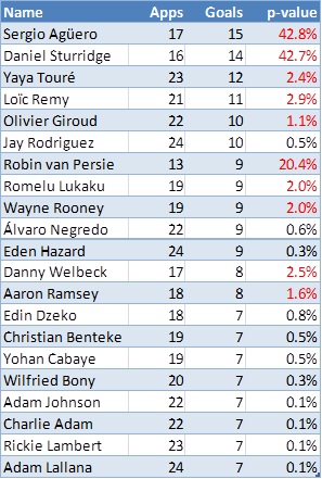 Red highlighted p-values show a total of 10 players whose scoring rate is not significantly different to Suarez at the 1% level of significance. So there you have it, some food for thought: perhaps surprising but Luis Suarez is no better than Sergio Aguero or even Danny Welbeck in terms of scoring rates, from a statistical perspective! [Finally, as promised for any interested parties, the p-value of this test is given by:
  where c1, c2 are the observed events (in the players’ example above, the number of goals) out of t1, t2 time periods (i.e. the number of appearances). c is defined as the sum of c1 and c2 while t is the sum of t1 and t2.] Reference: Przyborowski J., Wilenski H. (1940) Homogeneity of results in testing samples from Poisson series, Biometrika 31, 313-323
2014
Suarez, Aguero and the importance of significance
By Hudl Statsbomb
|
February 5, 2014
