As you may have read before, StatsBomb have an ongoing commitment to developing football analysts of the future. We try our best to provide the education, tools, and resources needed to learn the trade for the many amateur analysts out there looking to forge a career in professional football. Part of this commitment has been to release industry-leading event data free of charge, such as the recent FAWSL and Messi Data Biography data releases. Well, we have another one for you — one that we’re particularly excited about. Not just because Euro 2020 was a great tournament. For the first time, we’re releasing StatsBomb 360 data.
What is StatsBomb 360?
StatsBomb 360 is the next revolution in football event data. We revolutionised the industry already in 2018 with the launch of StatsBomb Data and its upgraded data spec. Amongst many other new features, the data spec included freeze-frames on shots to capture the location of all defenders, attackers, and goalkeeper at the moment of the shot. Well, StatsBomb 360 data captures a freeze-frame showing the location of all players in the frame for every event we collect.
360 will also allow us to uncover a host of new information about the game that was either difficult to see or completely hidden in standard event data. We will now be able to deliver things like:
- Line-breaking passes
- Ball receipts in space
- Distance to all defenders in the frame
- Passing lanes
- Defensive shape around every event
And that’s just the starting point of what will be possible with 360. Our clients have already started to increase their competitive edge with the extra depth this information provides, and we ourselves have been generating new ideas and insight every day, some of which was presented at our recent StatsBomb Conference.
Of course, if you just wanted to play with the standard Euro 2020 event data, then that’s ok. We’ve released that too.
Accessing the data
There are a few key things you’ll need to get started with the data. If you’re new to using StatsBomb data or just starting out on your coding journey, we’ve created a guide to using StatsBomb data in R to help you on your way, and created the StatsBombR and statsbombpy (for Python) packages to make working with and manipulating StatsBomb data that bit easier.
- Install the StatsBombR (if using R) or statsbombpy (if using Python) packages
- Keep the R Guide handy
- Keep the data specification handy
As this is the first ever release of 360 data, we’ll help you get started by giving an example of how to work with and gain insight from the data in R and create your first visual plot with it. It is recommended you work through the ‘Working With StatsBomb Data In R’ Guide first if you haven’t already, as the code and instructions we’re going to share here are aimed at more experienced users of the data.
Using StatsBomb 360 Data Case Study
The very first thing you’ll need to do is update StatsBombR. Delete the package, then run the line of code below to install the latest version of the package (assuming you already have it installed. If you don’t, refer to the R Guide for full installation instructions.)
devtools::install_github(“statsbomb/StatsBombR”)
In this example, we’re going to look at crosses, specifically how to calculate the number of attackers and defenders in the box at the time of the cross for each cross in the tournament. We’ll then select one of the crosses and show you how to plot the 360 frame to see the specific player locations at the event.
First, let’s pull the 360 freeze-frames and store them in a dataframe ‘data360’.
library (StatsBombR)
Comp <- FreeCompetitions()
Matches <- FreeMatches(Comp)
Matches = Matches %>% filter(competition.competition_name==”UEFA Euro”)
data360 <- free_allevents_360(MatchesDF = Matches, Parallel = T)
Next, we’re going to pull the standard Euro 2020 event data into a separate dataframe.
events <- free_allevents(MatchesDF = Matches, Parallel = T)
events <- allclean(events)
events <- get.opposingteam(events)
Then, we need to join the 360 frames to the respective events in the standard data, so we have both the standard event data and the 360 freeze-frames in one dataframe.
data360 = data360 %>% rename(id = event_uuid)
events = events %>% left_join(data360, by = c(“id” = “id”))
events = events %>% rename(match_id = match_id.x) %>% select(-match_id.y)
Now we can play with the data. From here, we want to find the 15 crosses that saw the most attackers and defenders in the box at the time of the cross.
We reduce the number of events in the dataframe to make the data a little easier to work with by filtering to Pass events and selecting only the variables we need for this exercise.
library(tidyverse)
ffs = events %>%
group_by(team.name) %>%
filter(type.name==”Pass”) %>%
select(id, match_id, team.name, OpposingTeam, player.name, type.name, minute, second, location.x, location.y, pass.end_location.x, pass.end_location.y, pass.type.name, pass.cross, freeze_frame)
Then we arrange the freeze-frames so that each player’s location is next to the corresponding event. ‘Unnest’ flattens the freeze-frame to parse each player’s location into an individual row within the dataframe.
ffs = ffs %>% unnest(freeze_frame) %>%
mutate(ff_location.x = (map(location, 1)), ff_location.y = (map(location, 2))) %>%
select(-location) %>%
mutate(ff_location.x = as.numeric(ifelse(ff_location.x == “NULL”, NA, ff_location.x)), ff_location.y = as.numeric(ifelse(ff_location.y == “NULL”, NA, ff_location.y)))
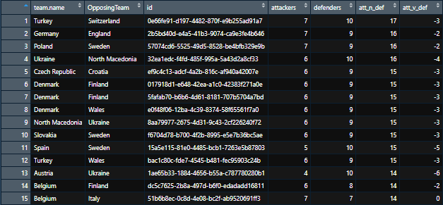
Finally, we create a new dataframe to filter to crosses that ended within the penalty area in open play and calculate the number of attackers and defenders in the penalty box at the time of the cross, as well as the total numbers of players in the box and the numerical difference between the number of attackers and defenders. We then sort the list by the total number of players in the box and display the top 15 results.
crosses = ffs %>%
filter(pass.end_location.x>102 & pass.end_location.y>18 & pass.end_location.y<62) %>%
filter(is.na(pass.type.name) | pass.type.name==”Recovery” | pass.type.name==”Interception”)%>%
filter(pass.cross==TRUE) %>%
filter(keeper==FALSE) %>%
group_by(team.name, OpposingTeam, id) %>%
summarise(attackers = sum(teammate==TRUE & ff_location.x>102 & ff_location.y>18 & ff_location.y<62, na.rm = TRUE),
defenders = sum(teammate==FALSE & ff_location.x>102 & ff_location.y>18 & ff_location.y<62, na.rm = TRUE),
att_n_def = attackers+defenders,
att_v_def = attackers-defenders) %>%
ungroup() %>%
arrange(desc(att_n_def)) %>%
head(n = 15)
The result should look something like this:

Now let’s plot the freeze-frame so we can see the exact locations of all the attackers and defenders within the frame.
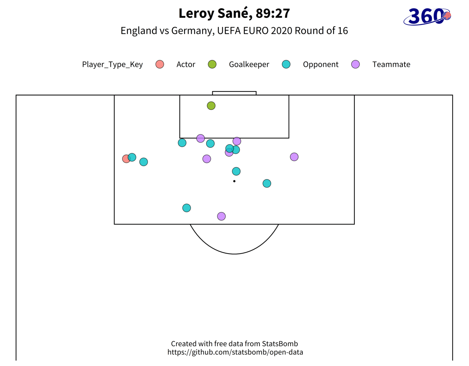
We need to filter the data we have in the ‘ffs’ dataframe to contain only the cross which we wish to plot, in this case let’s take Leroy Sane’s late cross vs. England that saw a total of 16 players (not including the keeper) crowd the area (the second option on the list above). We do this by taking the event id from our ‘crosses’ dataframe and pasting it into the code here. The ‘mutate’ function adds a new column to the dataframe, ‘Player_Type_Key’ that will form our key on the plot. This will distinguish the player making the action, the player’s teammates, opponents, and the goalkeeper.
chart = ffs %>%
filter(id==”2b5bd40d-e4a5-41b3-9074-ca9e3fe4b646″) %>%
mutate(Player_Type_Key = case_when(actor==TRUE & teammate==TRUE ~ “Actor”,
teammate==TRUE ~ “Teammate”,
teammate==FALSE & keeper==FALSE ~ “Opponent”,
keeper==TRUE & teammate==FALSE ~ “Goalkeeper”))
Now we can create the plot.
library(ggplot2)
library(grid)
ggplot() +
annotate(“rect”,xmin = 0, xmax = 120, ymin = 0, ymax = 80, fill = NA, colour = “black”, size = 0.6) +
annotate(“rect”,xmin = 0, xmax = 60, ymin = 0, ymax = 80, fill = NA, colour = “black”, size = 0.6) +
annotate(“rect”,xmin = 18, xmax = 0, ymin = 18, ymax = 62, fill = NA, colour = “black”, size = 0.6) +
annotate(“rect”,xmin = 102, xmax = 120, ymin = 18, ymax = 62, fill = NA, colour = “black”, size = 0.6) +
annotate(“rect”,xmin = 0, xmax = 6, ymin = 30, ymax = 50, fill = NA, colour = “black”, size = 0.6) +
annotate(“rect”,xmin = 120, xmax = 114, ymin = 30, ymax = 50, fill = NA, colour = “black”, size = 0.6) +
annotate(“rect”,xmin = 120, xmax = 120.5, ymin =36, ymax = 44, fill = NA, colour = “black”, size = 0.6) +
annotate(“rect”,xmin = 0, xmax = -0.5, ymin =36, ymax = 44, fill = NA, colour = “black”, size = 0.6) +
annotate(“segment”, x = 60, xend = 60, y = -0.5, yend = 80.5, colour = “black”, size = 0.6)+
annotate(“segment”, x = 0, xend = 0, y = 0, yend = 80, colour = “black”, size = 0.6)+
annotate(“segment”, x = 120, xend = 120, y = 0, yend = 80, colour = “black”, size = 0.6)+
theme(rect = element_blank(),
line = element_blank()) +
# add penalty spot right
annotate(“point”, x = 108 , y = 40, colour = “black”, size = 1.05) +
annotate(“path”, colour = “black”, size = 0.6,
x=60+10*cos(seq(0,2*pi,length.out=2000)),
y=40+10*sin(seq(0,2*pi,length.out=2000)))+
# add centre spot
annotate(“point”, x = 60 , y = 40, colour = “black”, size = 1.05) +
annotate(“path”, x=12+10*cos(seq(-0.3*pi,0.3*pi,length.out=30)), size = 0.6,
y=40+10*sin(seq(-0.3*pi,0.3*pi,length.out=30)), col=”black”) +
annotate(“path”, x=107.84-10*cos(seq(-0.3*pi,0.3*pi,length.out=30)), size = 0.6,
y=40-10*sin(seq(-0.3*pi,0.3*pi,length.out=30)), col=”black”) +
geom_point(data = chart, aes(x = ff_location.x, y = ff_location.y, fill=Player_Type_Key),
size = 6, alpha = 0.8, shape=21) +
theme(axis.text.x=element_blank(),
axis.title.x = element_blank(),
axis.title.y = element_blank(),
plot.caption=element_text(size=13,family=”Source Sans Pro”, hjust=0.5, vjust=0.5),
plot.subtitle = element_text(size = 18, family=”Source Sans Pro”, hjust = 0.5),
axis.text.y=element_blank(),
legend.position = “top”,
legend.title=element_text(size=14,family=”Source Sans Pro”),
legend.text=element_text(size=14,family=”Source Sans Pro”),
legend.margin = margin(c(20, 10, -65, 50)),
legend.key.size = unit(1.5, “cm”),
plot.title = element_text(margin = margin(r = 10, b = 10), face=”bold”,size = 24, family=”Source Sans Pro”, colour = “black”, hjust = 0.5),
legend.direction = “horizontal”,
axis.ticks=element_blank(),
aspect.ratio = c(65/100),
plot.background = element_rect(fill = “white”),
strip.text.x = element_text(size=13,family=”Source Sans Pro”)) +
labs(title = “Leroy Sané, 89:27”, subtitle = “England vs Germany, UEFA EURO 2020 Round of 16”, caption = “Created with free data from StatsBomb\n https://github.com/statsbomb/open-data”) +
coord_flip(xlim = c(85, 125))
Which should look something like this:

This code is intended to be a starting point to get you going with your analysis. Mess around with the event types, filters, and plots to create your own vis — the possibilities of what can be discovered with this data are significant, and we hope you have fun experimenting and discovering them.
Indeed, if you needed a little more inspiration, several presentations on the Research Track stage at our recent StatsBomb Conference presented research performed on StatsBomb 360 data. You can watch the talks here, which could help inspire more ideas and avenues to explore.
Best of luck,
The StatsBomb Team

