This article is co-authored by Yohahn Ribeiro and Alex Palmer-Walsh.
American football is a game of power, strategy, and precision. Behind the thrilling touchdowns and bone-crushing tackles lies a world of physical metrics that play a crucial role in determining a player's success on the field.
In this article, we will discuss how we're leveraging our high quality, human + AI generated, tracking data to compute physical metrics that will enable our customers to make even more informed decisions about their players and tactics.
Advanced Physical Metrics from Video Footage
In the ever-evolving landscape of sports analytics, traditional statistics can only tell part of the story. To gain a deeper understanding of player performance and team dynamics, coaches, analysts, and organizations are turning to advanced physical metrics.
What sets these metrics apart is their origin: they are extracted from the actual on-field action, captured through video footage such as broadcast and ALL22 views. This approach offers distinct advantages over relying solely on metrics from events like the NFL Combine.
While Combine metrics provide valuable data, they are often recorded in controlled settings and don't fully reflect a player's in-game performance. In contrast, data derived from video footage captures nuances such as a player's acceleration in a specific play or their ability to make rapid directional changes under real game conditions. This wealth of data from live gameplay enables decision-makers to make more accurate and context-rich assessments of player capabilities and tactics.
Tyreek Hill - Kansas City Chiefs vs Buffalo Bills (NFL Division Championship 21 / 22)
In the above Kansas City Chiefs vs Buffalo Bills game, you can see Tyreek Hill utilising his incredible agility and speed to change direction, catch the ball and leave the Bills defenders in the dust. Generating metrics for players and plays like this, directly from video footage, can be incredibly useful for comparisons and benchmarking; only enriching insights from NFL Combine data.
What Physical Metrics Are We Generating?
We're researching and developing various enriched player metrics for integration into our platforms, but for this article we'll focus on a few simple metrics we are developing. These quantities are intuitive and provide a good basis for initial development. Always good to get the basics right!
- Total Distance Covered: In the dynamic world of American football, players traverse significant distances during a game. The "Total Distance Covered" metric reveals the incredible stamina and endurance of players. Coaches can use this metric to assess a player's fitness level and determine if they can maintain peak performance throughout the game.
- Cumulative Distance: Beyond just the total distance, "Cumulative Distance" provides a historical perspective. It sums up the distance a player covers across a play, multiple plays or multiple games. This metric offers insights into a player's work rate over time, highlighting their consistency and ability to contribute throughout the season.
- Speed: Speed is a fundamental metric that transcends all positions in football. It's not just about who can run the fastest in a straight line; it's about who can reach their top speed quickly and then maintain that speed. It's an essential metric for evaluating wide receivers racing to catch a pass or defensive backs trying to close the gap on a sprinting opponent.
- Max Speed: "Max Speed" identifies the highest velocity reached by a player during a play. This metric is particularly valuable for assessing explosive acceleration and bursts. It reveals those lightning-fast moments when a player shifts into high gear, often making the crucial difference between a touchdown and a tackle.
- Acceleration: In the sport of quick decisions and rapid reactions, "Acceleration" is king. This metric measures how swiftly a player can go from a standstill to top speed. It's essential for understanding a player's agility and ability to change direction on the fly. Running backs who burst through a gap in the defence or line-backers who close in on a ball carrier rely heavily on their acceleration.
- Max Acceleration: "Max Acceleration" pinpoints the highest rate at which a player can change their speed. It's about those split-second bursts of energy that leave defenders flat-footed. This metric helps identify players who excel in evading tackles or making explosive cuts.
From High Frequency Location Data to Higher Order Metrics
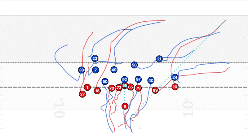
At StatsBomb we leverage various AI and Computer Vision techniques to generate high frequency tracking data. This data is then carefully audited by our incredible team of collectors using in-house developed collection apps.
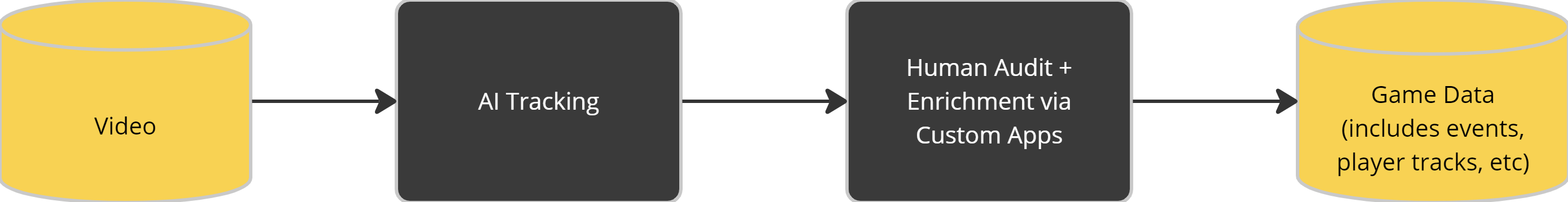
Briefly, the AI Tracking system first retrieves all the frames for a play (a video segment). The next step is to generate homography and object detections for all frames. All this information is then processed by a tracking algorithm that links detections across frames into “tracks” i.e. identifying players throughout the play.
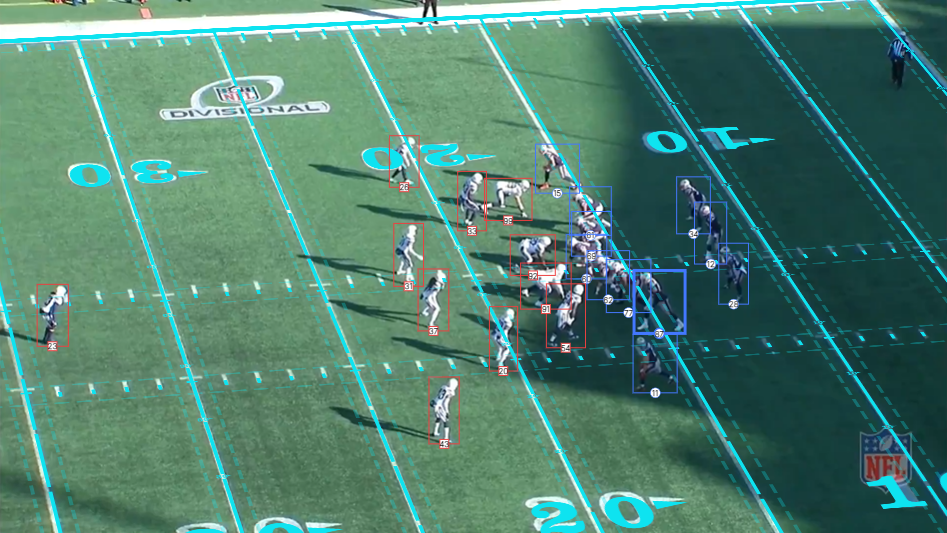
AI Generated Outputs in Custom Track Collection App
The player tracks along with the estimated homography information is combined to estimate the actual pitch positions for all players in the play. A full description of the tracking system will be the subject of a future blog post.
AI Generated Tracks in Custom Track Collection App
The tracking system generates data for every frame in a broadcast / all22 play. This allows us to calculate a player’s metrics with high granularity, offering greater insight and aiding analysis.
Smoothing Raw Tracking Output
Any measurements taken from a sensor will contain some level of sensor noise. Sensor noise is any variation in sensor readings that does not reflect the true state of the phenomenon being measured.
In the case of player tracking, some sources of sensor noise are the AI models we use to detect the homography and player positions.
Given an input video frame, the player detection model will detect a bounding box around a player. When we run the model on the next frame in the video, the bounding box may not be in exactly the same place as before, even if the player hasn’t moved.
This slight movement of the box from one frame to the next is what we call "bounding box position noise." It's like a small wobble or jitter in the box's position caused by the way the player detection model works, resulting in jitter in the final player pitch position.
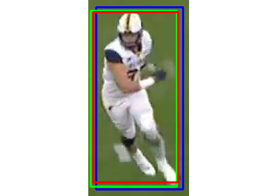
Example of bounding box noise.
To account for this noise, we apply a smoothing filter to player x and y pitch positions over time. Various smoothing methods can be used for this, such as moving mean, a low pass filter, Kalman filter and others.
As seen in the figure below, the output of the smoothing filter is a signal with reduced noise. We can adjust the parameters of this smoothing filter depending of the level of noise we wish to filter out.
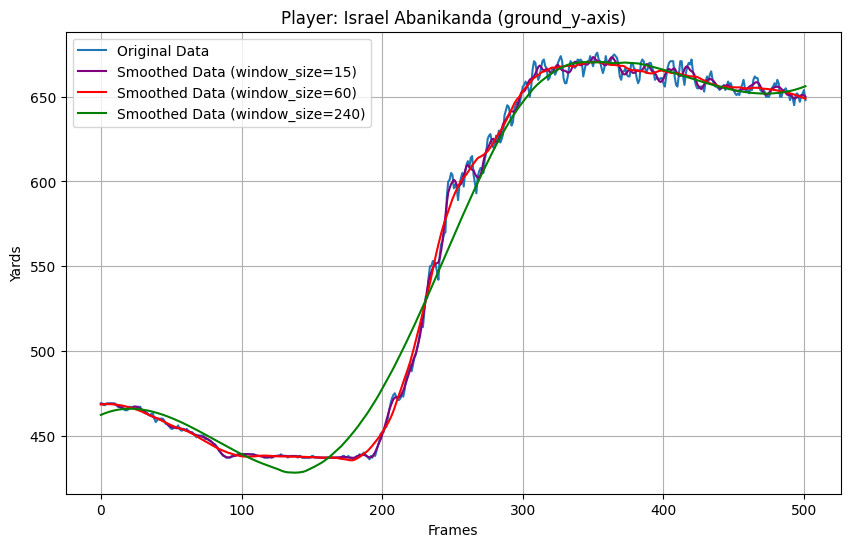
Smoothing filter applied to player y position
It is important to note that depending on the configuration of the filter used, the smoothed signal may deviate from the underlying “true signal”. We are aware of this and are conducting ongoing research against ground truth datasets in order to increase confidence in the smoothing strategy.
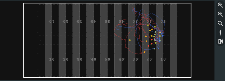
Player Track Segments
When generating metrics from video footage, we face a limitation when players move off-screen and then return into view. This is a common occurrence in broadcast video for example. To address this, we employ a straightforward approach. We simply identify when a player goes off-screen and calculate metrics solely for their on-screen segments.
This is accomplished by analysing the video's frame rate or frames per second (FPS) and the timestamps in a player's positional data. When a player remains on-screen, their positional data aligns closely with the video's FPS. This is not precise due to minor timestamp variations related to floating point errors and non-constant frame rates. A threshold is employed to handle these fluctuations.
In contrast, when a player goes off-screen, there are significant timestamp gaps, allowing us to define distinct "player segments" for metric calculations.
StatsBomb Generated Examples
Here are some examples for long run plays using the tracking data and smoothing techniques outlined above.
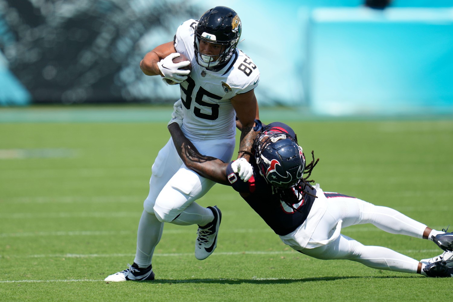
Israel Abanikanda - Physical Metrics
Brenton Strange - Physical Metrics
Julian Fleming - Physical Metrics
The visuals above provide a per timestamp / per frame display of the captured metrics. However, the entire velocity and acceleration signals for all players can also be visualised.
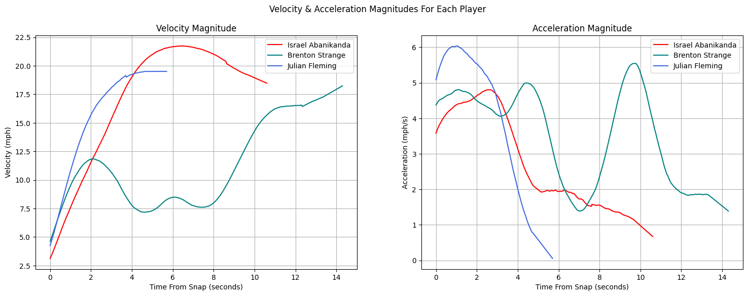
Velocity and Acceleration Signals for All Players
This type of high frequency metric data coupled with in-game context, derived from event and video data modalities, provide a more nuanced view of player performance. Metrics can be measured and analysed over the entire duration of a play, breaking away from the summary statistics that may mask important details.
For example, Brenton Strange has a fairly complex velocity profile as he receives the pass near the side-line and dodges several tackle attempts. This may be more valuable than simply hitting maximum speed in a play.
Conclusion
As we’ve seen physical metrics from video can be extremely beneficial, providing contextual information from in-game scenarios. In this article, we’ve outlined some basic preliminary physical metrics we’re looking into at StatsBomb, and some of the issues we’ve faced along the way.
We have many exciting metrics on the roadmap. However, our next step is to validate our metrics generation process alongside some of our partner clubs and industry provided NGS data, to ensure we maintain high levels of reliability and quality.
If you want to discuss any of the themes or ideas touched upon in the article, feel free to connect with our Machine Learning Engineers and authors of the piece Yohahn Ribeiro and Alex Palmer Walsh.
