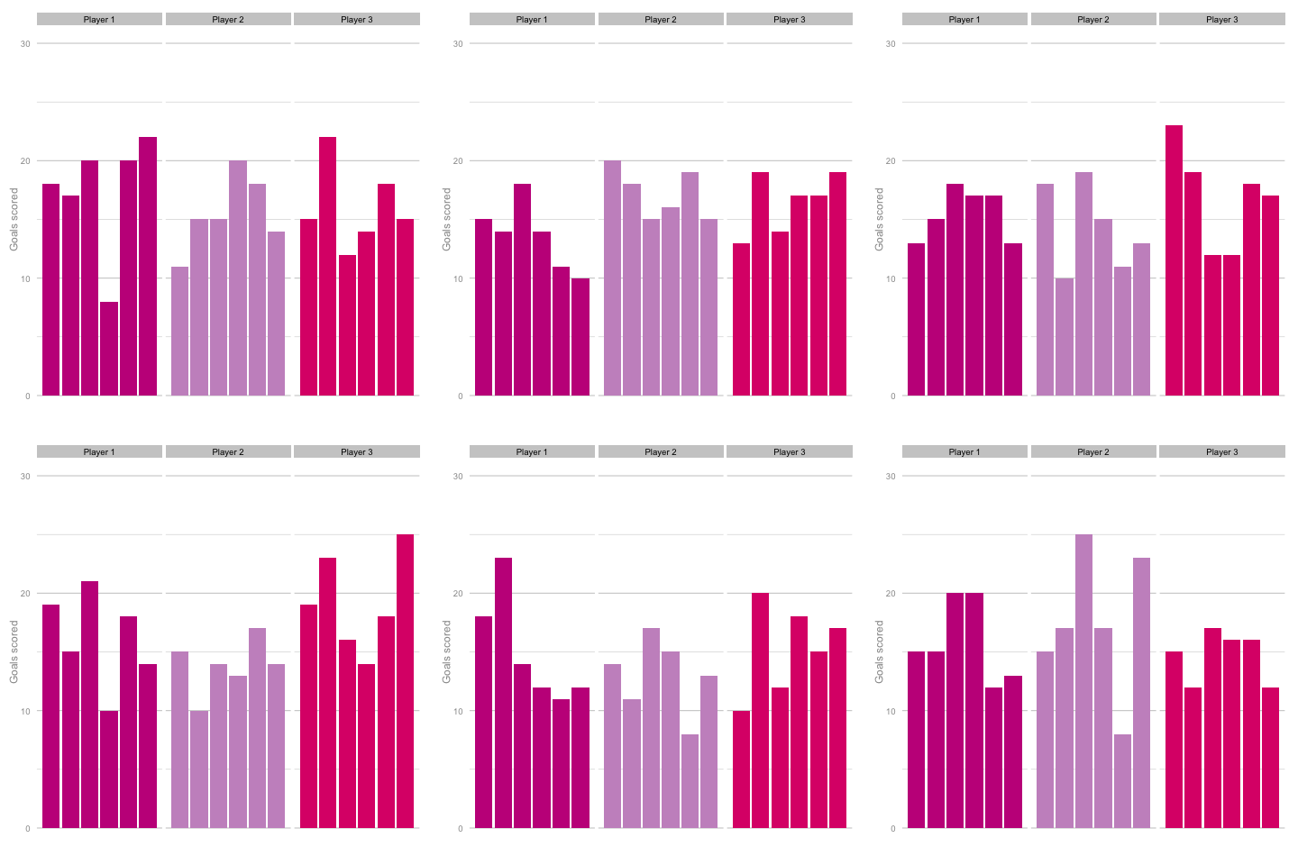
Short termism is rife in football coverage these days. From the insatiable desire to learn 5 things from each match day to the pendulum swing in Falcao’s perceived talent level between last summer and this. It’s common to hear strikers’ peaks and troughs talked about in terms of confidence, hunger and desire, as though each change in output is the result of some tweak in the internal machinery of the player’s mentality and training. But how much of this is true and how much can be attributed to statistical noise? Take these three players, for instance. Goal-scoring in 6 consecutive season adjusted for minutes played. Who do you think they are? Which player is the best?  Of course, as you may have guessed from the article so far, this is a trick question. They are, in fact, the same player (sort of). These charts are the results of three simulations using the same starting conditions. These three 'players' are taking the same number of shots (138) with each shot being given the same probability of being scored (14%) for each of the 18 seasons shown. With this in mind it’s easy to see how narratives can form from little more than random variation. Is player 1 in decline? Is player 2 more consistent than the other players? Of course, it’s easy for me to be smug having shown just one comparison. Below is a gif cycling through more simulations using the same starting conditions as above.
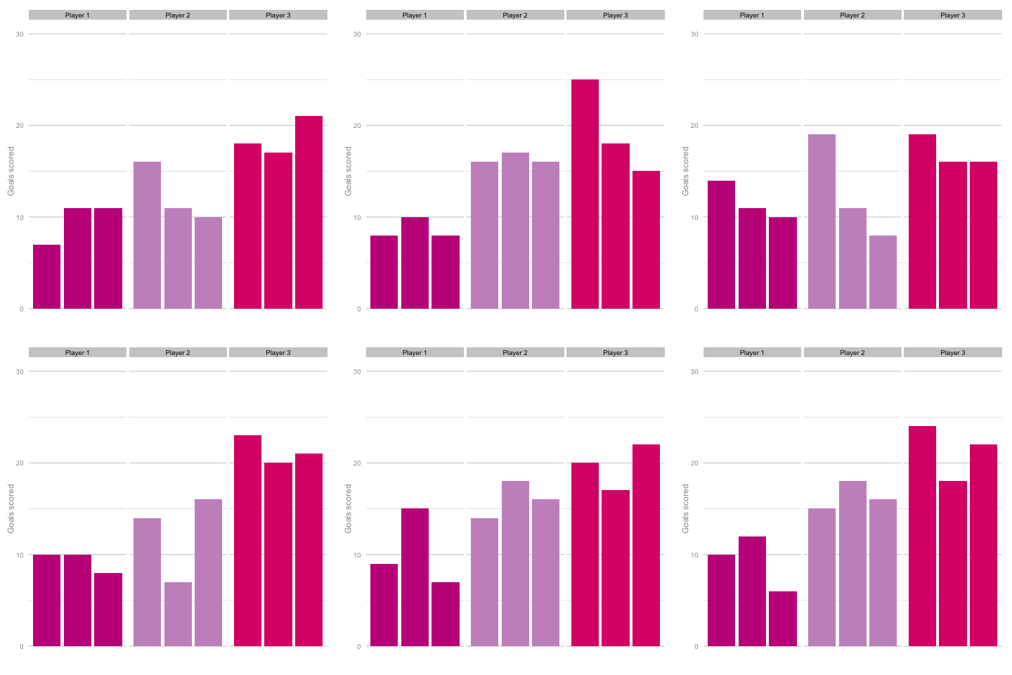
  Unsurprisingly, most simulations don’t seem to suggest a wild difference between each player’s output over the 6 simulated seasons. Nonetheless, it can be tempting to see patterns in individual frames. Perhaps a player looks like they’re steadily improving, for instance. Maybe one player looks consistent, while the others are unpredictable or mercurial. If we were to add in real world events around these virtual players, and it's easy to see how we can be tricked by randomness. That freak 25 goal season could start to look like the new manager’s stroke of genius. Or maybe that slump to 10 goals coincides suspiciously with some off-field revelations in the tabloids. In a slightly different example, what if the players were performing differently? How easily could you tell? The following set of simulations shows the three players taking a different number of shots, (though each individual shot continues to have the same probability of being scored). In this example, the players are taking 70, 100 and 130 shots. Over a 2000 minute season (22.2 90s), this corresponds to a difference of 1.35 shots p90 (or, if you prefer, roughly one 14/15 Ashley Young) and a difference of 4.2 expected goals (30 shots * 14% chance of scoring each).
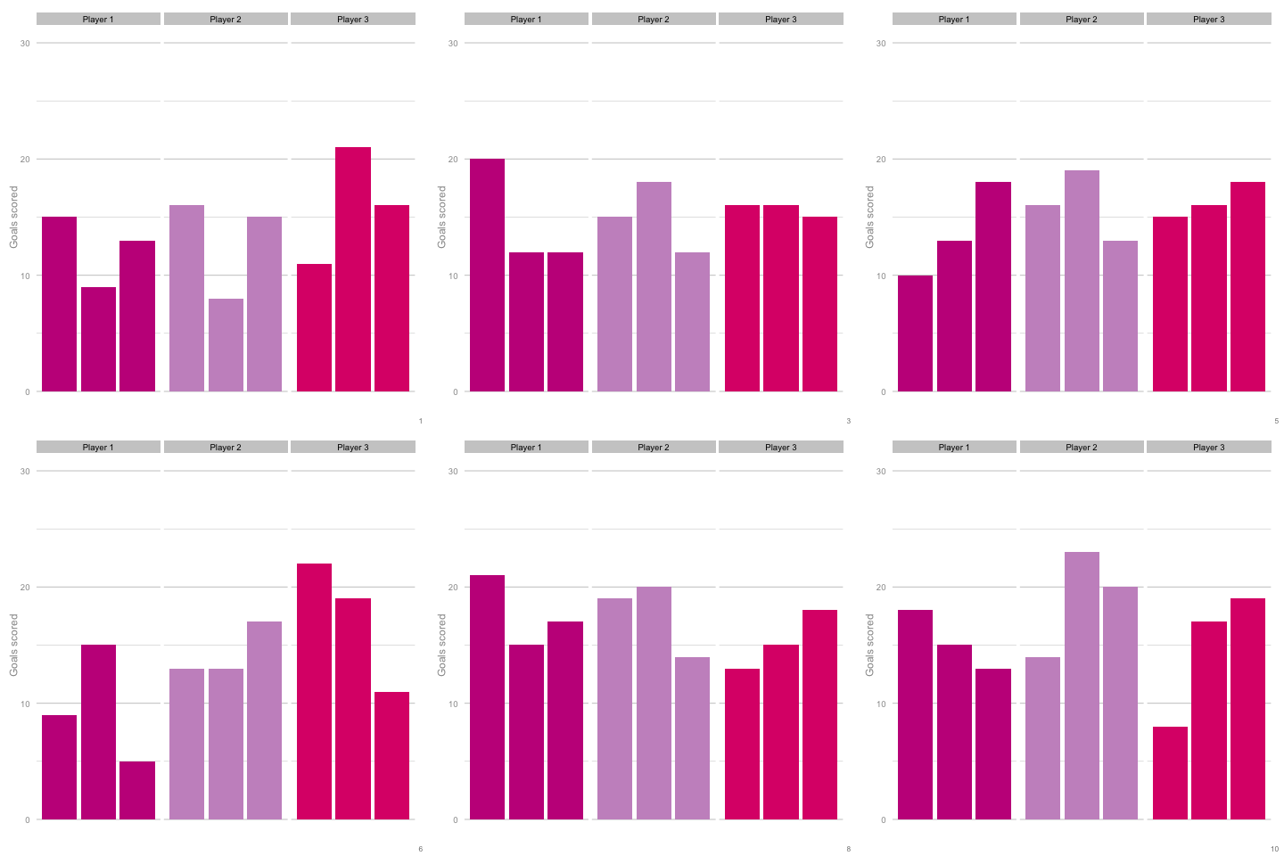
  It’s pretty easy to see which player is which after a few frames. Nonetheless, we can also see how this difference in players can be exaggerated or eliminated by nothing more than variance. Moreover, each frame is a top down look at 9 seasons of (simulated) data, with no extra adjustment needed for minutes played, injuries, tactics or any of the other myriad factors that go into a real season of football. The 'true' difference between players in an individual simulation can be masked by randomness. The final gif shown is a combination of the previous two. It shows 10 frames: half of them have identical starting conditions and the other half are graded as in the previous example. Can you tell which is which?*
  In the real world, clubs can’t just run another simulation to get a better idea of who’s actually good. Randomness and probability are really hard; real world events are unpredictable and irregular. This is where analytics is useful, from fans and media outlets, to coaches and managers. By creating models and looking at the underlying numbers, we can identify where random variation is strongest, react and move to make fewer mistakes or eliminate rash decisions as a result. For instance, in this example, moving from goals to a closer look at the shots numbers would give a clearer idea of whether the differences in these players' performance was likely to be repeatable. We can then use models and perform statistical tests to get a better idea of how likely it is that one player is superior to another. For clubs, this can be used as a complement to more traditional recruitment techniques to avoid costly overpays on over performing players, or to find bargains. For fans, knowledge of such numbers can help avoid results-driven hysteria and see that it's more likely that Arsenal are still quite good (but perhaps unlucky) and that Chelsea really have been that bad. Credit to NY Times (http://www.nytimes.com/2014/05/02/upshot/how-not-to-be-misled-by-the-jobs-report.html?_r=0) and Lena Groeger's talk (https://www.youtube.com/watch?v=zd0YQAgu3dI) for the dataviz ideas that this article shamelessly appropriates. *Seasons with the same starting conditions: 1, 2, 3, 8 and 10 (number shown in bottom right corner)
2015
Randomness And The Fog Of Goals
By admin
|
September 7, 2015