Introduction
Expected goals (xG) is one of the oldest concepts in football analytics, introduced at least three decades ago. Since football is a comparatively low scoring game, the number of goals scored by a team varies considerably based on how a few situations play out. The idea of trying to determine how many goals a team or player should have scored, on average, from one or more situations is therefore an intuitive way to analyse team and player performance by minimising the variability from simply looking at outcomes for a handful of events.
Quantitative researchers in football have been well aware of the benefits of using xG instead of observed goals for performance analysis for some time. It’s known to be a better predictor of future performance than observed goals at both the team and player level. In fact, big clubs have been making decisions on which players to sign partially influenced by players’ xG values for a while, including Liverpool’s decision to sign players like Mo Salah.
More recently, the idea of xG has broken free from the data analyst circles to become part of how pundits and fans discuss the game. Just a few weeks ago, we saw Jamie Carragher discussing goalkeeper’s goals saved above expectation on Sky Sports. End-of-season league table forecasts from models, which rely on expected goals, are also becoming part of popular discourse, particularly around the chances of teams winning the title race, tracking the relegation battle, or fighting for a Champions League spot.
With the increasing acceptance of xG, it is important to remember that the expected goal rate for any given shot isn’t a universal value. xG is a concept - it is a model’s estimate of the number of goals that would have been scored, on average, from a situation or a collection of situations.
Especially relevant to today, not all xG values are created equal. Different models can vary enormously in how much data they consider, or how that data is modelled. The xG models are only as good as the data used to train them, and the design decisions and assumptions underpinning the model. Most developments in xG have been the inclusion of richer contextual data that has become available. The high-level concept of how these models are trained and used have remained comparatively stagnant since the early days.
As a result, we have decided to take a step back and look at areas in which the models can be improved to bring some much-needed innovation. This delivers a rich new lens through which we can understand teams and players’ performance. Today is a preview of how our new models show that there’s a lot of untapped potential left in this simple foundational concept.
Let’s look back to what we said when we released Shot Impact Height to the football world:
“Since StatsBomb Data debuted in 2018, StatsBomb expected goals (or xG) has always been a little bit different. The vision with SB Data was to transition football data from the world of proxies into a more accurate reflection of what is actually happening on the pitch. Right out of the gate, we added the location of goalkeeper and defenders around a shot, on every shot, in every league that we collect. This seemingly small upgrade delivered substantial improvements measuring xG numbers in densely packed penalty areas and especially when the GK is out of position.
Combine better xG numbers with pressures, pass footedness, a host of other USPs, and an overarching emphasis on quality and accuracy in the data, and it’s easy to see why StatsBomb Data has become the default choice for smart teams, federations, and gamblers everywhere. Our data is more accurate not only for where events occur on the pitch, and in what order, but it’s also more accurate regarding when events occur. That means that StatsBomb data is easier to effectively merge with tracking data than any other event data on the market.”
These seemingly small improvements to xG models - which were the result of massive data improvements - continue to deliver the best expected goals numbers in the business. Fans seem to agree, because every time someone releases a new xG model, even if it’s Amazon or Microsoft, they tell the social media world how ours seems to better reflect the quality of each chance.
We set the bar… but still felt we could do better.
StatsBomb xG, Summer 2022 Upgrade
There are upgrades all over, but the new features have resulted in significant upgrades to goalkeeper metrics and evaluations, as well as improving the viability of post-shot xG as a measure of a player’s finishing skill:
- The new model has an improved response to blocker and/or goalkeeper positioning
- Improved reliability in long shots and shots from particularly unusual situations
- We now have a better understanding of goalkeeper positioning and its contribution to suppressing xG values
- Understanding of finishing skill is improved via the decoupling of chance quality and shot execution
- Shot Velocity is now a feature in our Post-Shot xG model
- These upgrades will be available in StatsBomb data - live and post-match - later this year, covering all of our historic data and everything we collect going forwards
Let’s dig deeper into the modelling work performed in recent months to get to this point, and a preview of what we’ve found in evaluating goalkeeper positioning and finishing skill.
Model design decisions
Non-continuous features
“The new model has an improved response to blocker and/or goalkeeper positioning”
Right now, our existing xG takes into consideration the location of off-ball players freeze frames at the time shots are taken:
- the number of blockers in the triangle between the shot-taker and goalposts
- the proportion of the goalface blocked by the defenders
- whether there is any player between the goal and the shot-taker (the open-goal feature)
However, some of these features are discrete in nature. The number of defenders blocking the goal is an integer and can only increase/decrease in steps of 1. The open goal feature is a binary feature which can only be True/False. Features that can only move in discrete steps have some implications in how the model behaves for cases where the shot situation represents a borderline case.
Let’s consider what happens to models similar to our existing xG models as we drag the goalkeeper across a line that blocks different parts of the goalface.
We see a big discontinuity in xG when the goalkeeper is on the edge of the triangle between the shot-taker and goal because on one side of that boundary, the situation appears like an open-goal situation, or as the goalkeeper not blocking the goal. This is problematic because we know that in practice, a tiny change in goalkeeper position doesn’t result in such a dramatic change in real goalscoring likelihood. This phenomenon applies to other features too such as the location of opposition players, where moving any potential blocker just in/out of the triangle results in a step change in the number of blockers to goal, which results in a step change in the implied xG of the situation.
This problem can be overcome by replacing non-continuous features where we expect the relationship between that feature and goalscoring rates to be smooth. This applies to any features that rely on the location of players or are derived from them e.g. the open-goal feature. We achieve this by representing defenders as 2D bell-shaped surfaces (2D Gaussian distributions) instead of fixed-radius circles.
As a result, we can now measure partial blocking if the blocker is near the shot-taker-goalposts triangle i.e. the blocker could still block the goal, but it’s less likely than if the blocker were firmly in the shot-taker-goalposts triangle. A consequence of this is that the extent to which a player blocks the goal becomes a continuous number that gradually transitions from 1 to 0 as a blocker moves away from the shooter-goalface triangle.
This results in a much more intuitively-behaved model, as can be seen in the animation below.
A similar process can be applied to the projection of the blockers onto the goal face to obtain a “soft” and smooth goal-face occlusion array/feature, which will have similar improvements:
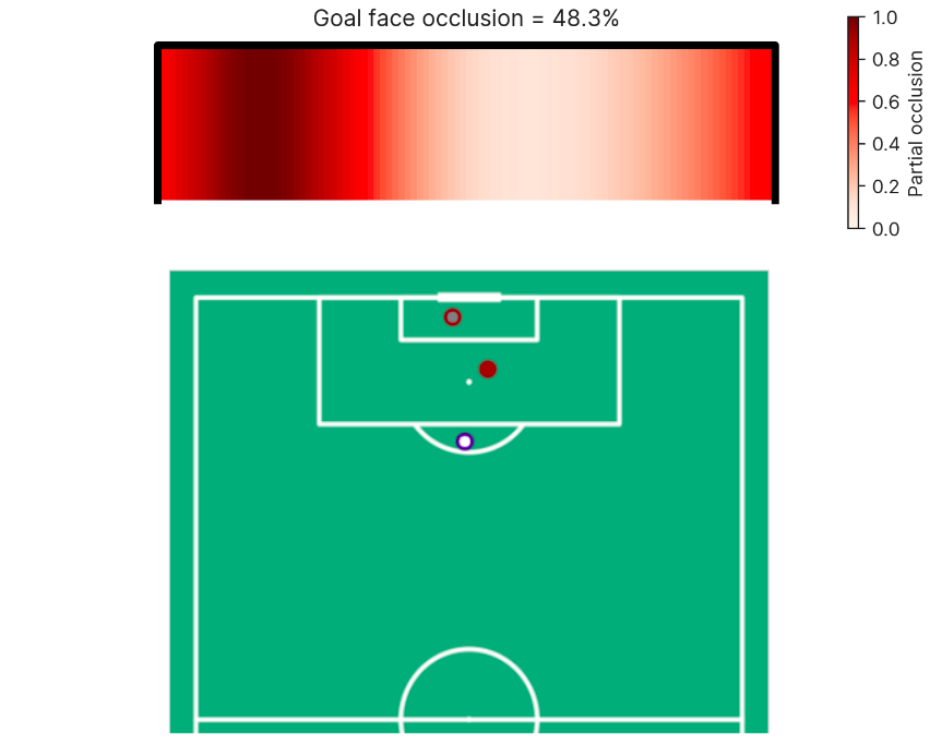
When training models with these features, the relationship between the feature and the expected goal rate ends up becoming considerably smoother. This has the advantage of being a closer representation of how the real probability of goal changes in response to small changes in player location.
This is especially important since the location of players in freeze frames will have some uncertainty associated with them, and the uncertainties in implied xG that arise from the uncertainties in player locations will be considerably smaller for these newer models as a result of the smoother relationships and continuous features.
Monotonic feature relationships
“Improved reliability in long shots and shots from particularly unusual situations”
Our xG models are Gradient Boosted Trees models. They are designed to learn patterns present in the data, but the models have no knowledge of what a real underlying relationship is between a feature and goal rates (signal), or artifacts from stochastic measurements (noise). As a result, it is not uncommon for models to sometimes end up looking a bit jagged as they “learn” some of the relationships caused by the noise in the data along with the real underlying relationship between the features and the target.
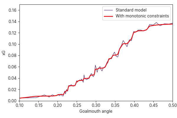
This problem can be partially overcome with some regularisation in the model, but there are other approaches available to allow us to inject some real world knowledge about the expected nature of the relationship between features and the target. We know that, with all else being equal, the likelihood of scoring will decrease as the visible goalmouth angle decreases (implying a tighter shot angle or greater distance from goal). We can add monotonic constraints to the model so that the learned relationships can only go in a single explicitly-stated direction.
The example below shows the relationship between goalmouth angle and goal likelihood for open play shots taken with the foot, comparing models with and without monotonic constraints to illustrate the phenomenon, and how monotonic constraints result in smoother and more intuitively-behaved relationships between features and the goal rate.
In our new xG models, we have replaced features with non-monotonic relationships with goalscoring likelihood. For example. the shot location y coordinate, where as we move from across the width of the pitch (from y=0 to y=80), the expected goal rates initially increase with the y coordinate as we get more central from the left edge of the pitch, but past the middle of the pitch (y=40), the expected goals start to decrease again with the y coordinate as we get to the right edge of the pitch. The overall relationship between the y-coordinate and expected goal rate is therefore U-shaped.
These have been replaced with variants that encode similar information, but that have a monotonic relationship with goalscoring likelihood e.g. distance and angle to goal, which allows us to include appropriate monotonic constraints in all features where the expected relationship is known and firmly uni-directional. This means that for any given situation, our post-shot xG model will only ever increase if a shot is placed further from a goalkeeper (as long as it’s still on-target) and the goalscoring probability will only ever increase as the shot velocity increases (yes - our new post-shot xG models now include shot velocity!), among other similarly intuitively behaved feature relationships.
Benefiting from training several variants of models
“We now have a better understanding of goalkeeper positioning and its contribution to suppressing xG values”
There are several benefits we can obtain from training subtle variants of similar models by carefully adding or removing some features.
Let’s consider two variants of an xG model where one includes the position of the goalkeeper, and the other doesn’t. The version without the position of the goalkeeper will result in an estimate of xG by implicitly assuming average goalkeeper positioning for shots from that location and play context, because the model has no way of knowing where the goalkeeper actually is. A version of the model with identical features + goalkeeper position features, will have a similar xG estimate, but will deviate slightly in response to the actual location of the goalkeeper.
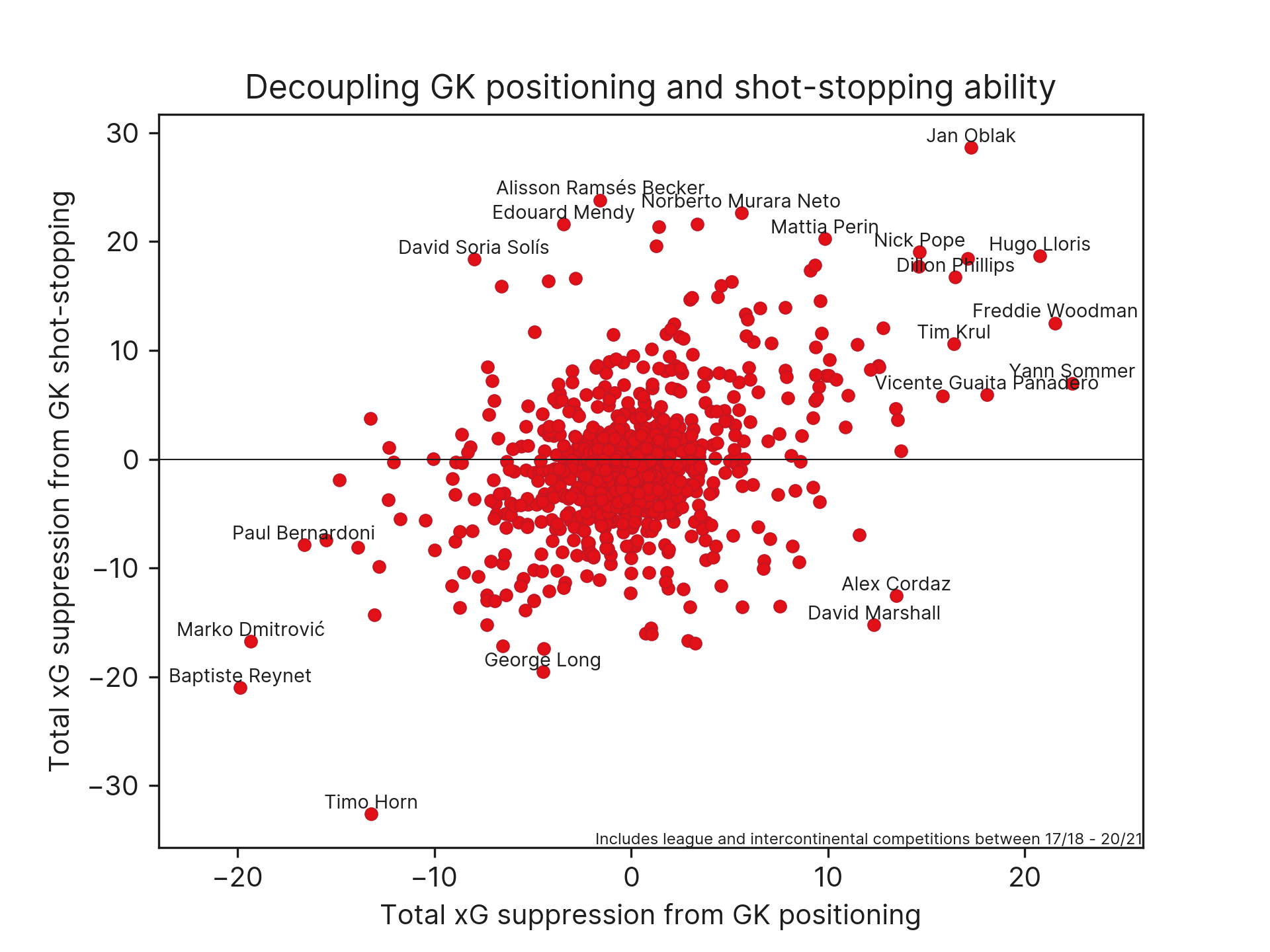
By taking the difference in xG estimates between these models, we can estimate how much higher/lower the xG of a situation is as a result of the goalkeeper’s position compared to the average GK position for that situation. This allows us to value GK positioning explicitly and decouple it from GK shot-stopping ability.
That said, it’s worth noting that while there are clear benefits to being able to decouple the value keepers add from their positioning choices in this manner, there are still some limitations to this approach. This approach only values the goalkeeper position at the instantaneous moment of the shot. Therefore, any goalkeeper positioning decisions that would force a shot to be taken from a comparatively unfavourable situation will be undervalued by this approach.
One example of this is 1v1 situations where a rushing goalkeeper forces an early shot. This approach is unable to take into account the fact that the shot will have likely been taken from a much more threatening location and context were it not for the GK’s positioning forcing the shot-taker’s hand. It’s therefore unable to properly assess the trade-off between maximising shot-stopping likelihood and forcing a shot from a less favourable situation, and will tend to slightly overestimate the positional value for goalkeepers who favour staying on their line and penalise GKs who force early shots in 1v1 situations e.g. Alisson. Fortunately, this mostly impacts 1v1 situations, which make up a comparatively small proportion of all shots, so this approach is still able to provide us with a good high-level estimate of goalkeepers’ positioning and shot-stopping abilities with larger sample sizes.
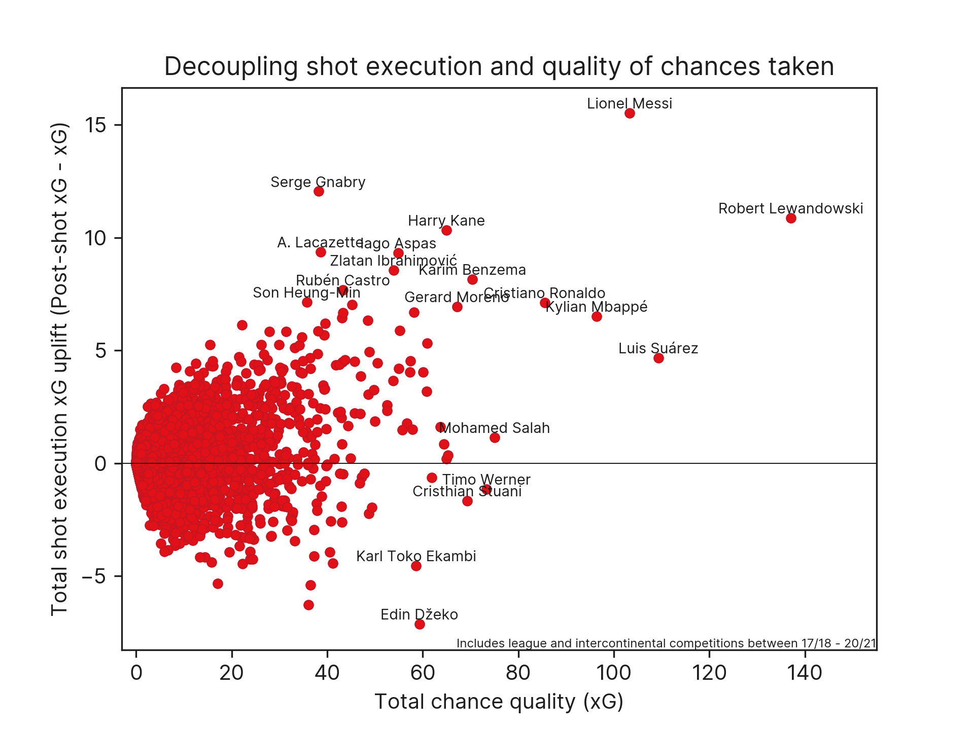
“Understanding of finishing skill is improved via the decoupling of chance quality and shot execution”
“Shot Velocity is now a feature in our Post-Shot xG model”
Similar to the idea of comparing xG models with and without goalkeeper location information, if we consider the difference in xG values between a chance quality model (which describes how dangerous a shooting opportunity is, considering the location of the goalkeeper and defenders) and a shot execution model (includes all of the above + shot placement and velocity), we get a measure of the estimated increase or decrease in goal probability from shot execution characteristics — the placement and velocity of the shot. This can be used to assess players’ execution ability, separate from the overall xG generated by a player by shooting from dangerous situations.
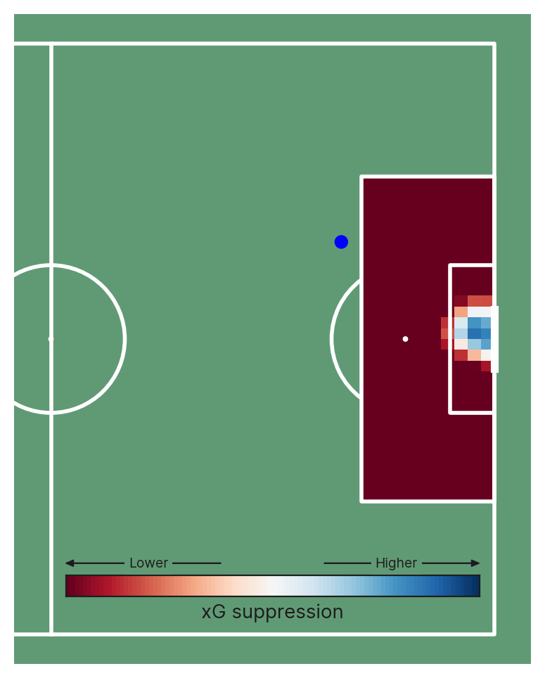
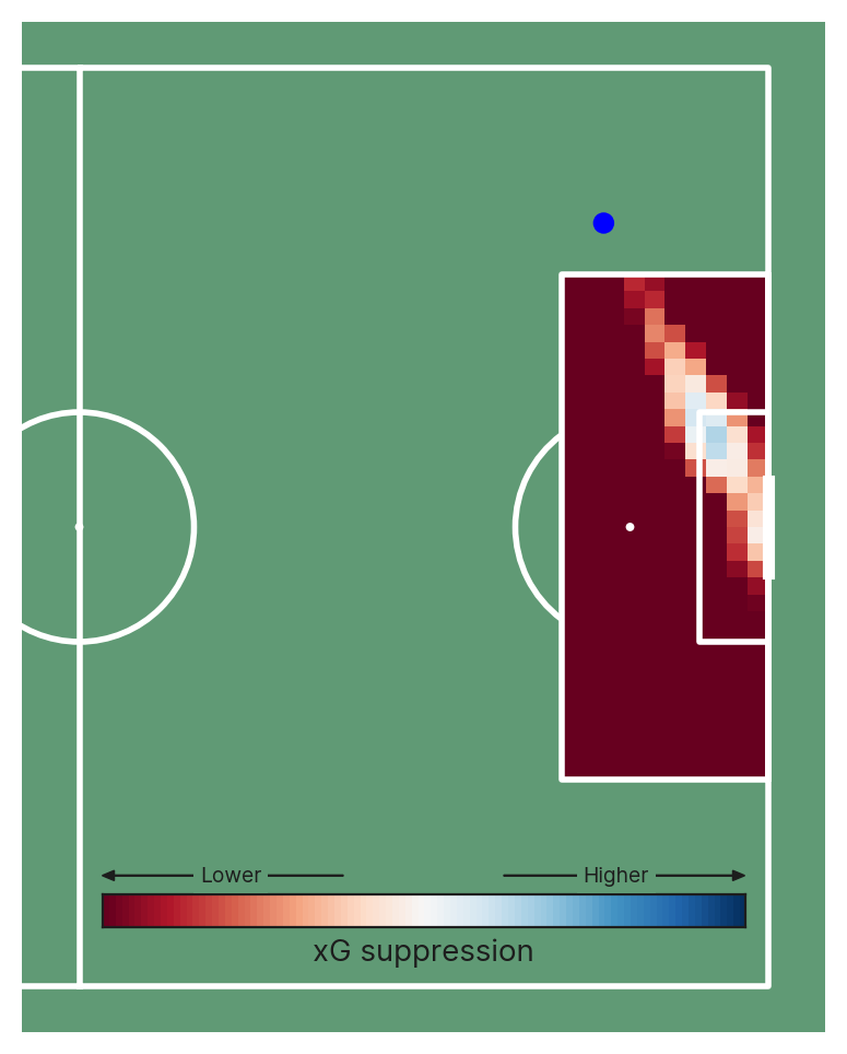
Insights from counterfactuals
The models we train are designed to estimate the goalscoring probability. Typically, we pass data for observed shots into the model to obtain expected goal likelihoods. This is of course very useful, but it can also be informative to generate the features for the counterfactuals (possible shots/situations that could have been, but weren’t the observed shot/situation).
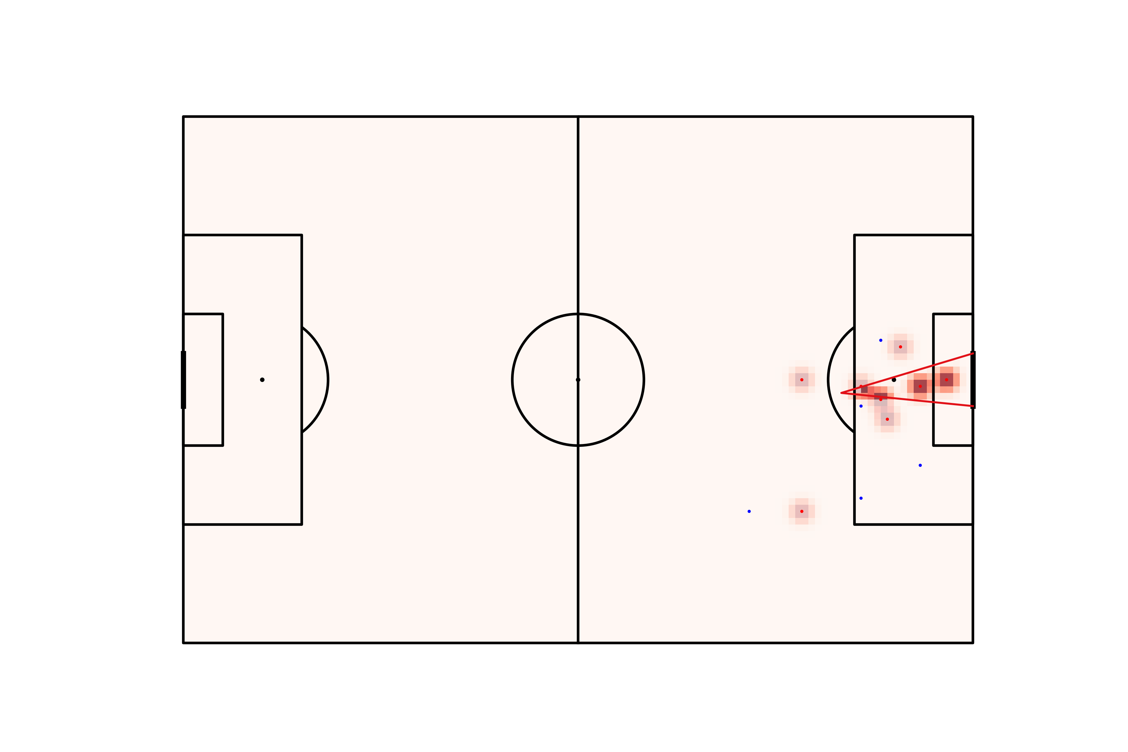
One example of this is GK positioning. We can generate and display the GK positioning value for the hypothetical situation where the GK was positioned in different areas of the penalty box to see how far off the optimal location the GK was situated. This can be useful since we may be interested in measuring GK positioning optimality in xG terms (how much better or worse than average the xG was as a result of the goalkeeper’s position), or in terms of spatial separation (how far off the optimal location the GK was located). Below are a few examples of how the GK’s positioning impacts xG.
A second example is shot execution. We can estimate the goalscoring likelihood if the shot was placed anywhere along the goal face. This can inform us on whether the shot placement was optimal, or how far off optimality a particular shot was. In simple cases, this may be obvious since shooting towards the corner of the goal furthest from the goalkeeper is the optimal shot, but becomes non-trivial if there are defenders blocking that shot path.
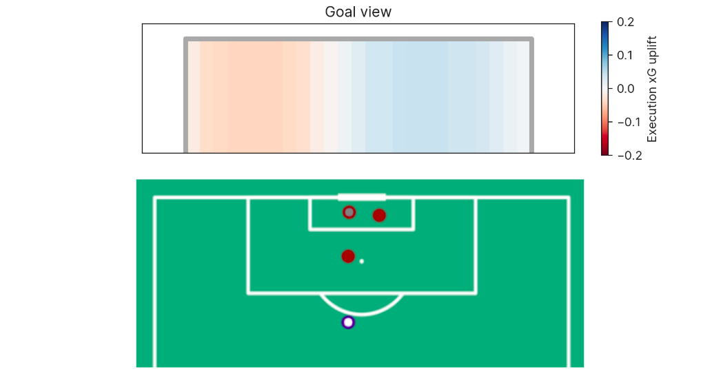
The shot execution xG added surface is, of course, also dependent on shot velocity.
Conclusion
The concept of xG is one of the oldest in football analytics. Despite that, there are still many improvements that can be made to these models to make them behave more intuitively, make them more resilient to small changes in the location of players, and unlock more insights into players’ and teams’ strengths and weaknesses in shooting situations.
We’ll be releasing a new xG model in the coming months with the key features discussed in this article:
- The new model has an improved response to blocker and/or goalkeeper positioning
- Improved reliability in long shots and shots from particularly unusual situations
- We now have a better understanding of goalkeeper positioning and its contribution to suppressing xG values
- Understanding of finishing skill is improved via the decoupling of chance quality and shot execution
- Shot Velocity is now a feature in our Post-Shot xG model
Every shot includes several xG-related outputs:
- Chance quality (xG)
- Shot execution (post-shot xG from the shot-taker’s perspective)
- Save difficulty (post-shot xG from the keeper’s perspective)
- Shot execution xG suppression
- GK positioning xG suppression
- GK shot-stopping xG suppression
- Shot placement xG maps
- GK positioning xG maps
