StasBomb’s exclusive line battles data provides tremendous detail on the interactions between the offensive and defensive lines. Via this data, we now know who each player engaged with, where they were on the field when this happened, and when/where the engagement both starts and ends. This in turn allows for the creation of metrics and analysis on vital areas of game planning and prep such as run tendencies, while also allowing deeper analysis- such as this look at pockets using our free TB12 data.
Run blocking is a key component of offensive line play. Linemen block defensive players in a manner coordinated to help create space for ball carriers to exploit. Depending on the run concept being used for a play, each player will have a different assignment. While the possible assignments are nearly unlimited, they can be categorized into one of several different block “types.” By identifying these block types at the individual player level on every running play, we can both begin to understand if certain players perform certain tasks better than others while also creating the building blocks for identifying run schemes and ultimately play calls themselves.
Our line battles data is intended to help the analysis of both individual player performance and team schemes and tendencies. The first step is the identification and assignment of those block types. In this article, we’ll go over how we managed it.
To model, or not to model: that is the question
As a data scientist, it is tempting to think that complex statistical models can solve everything. However, they are not always the answer. Sometimes simplicity and explainability are paramount.
Our aim is to attribute one of seven different block types (Base, Drive, Reach, Pull, Slice, Double Team, Second Level) to each offensive line player on each running play. In data science terms, this means training a classifier with seven different outcomes. While there are no issues with this statistically (many classification algorithms can successfully handle predictions for this many outcomes), modeling this data successfully comes with its own challenges.
Broadly speaking, there are two categories of machine learning models. The first category, supervised learning models, use labeled data to train the model. We don’t currently have labels for block type and collecting the number of labels we’d need would take a lot of time and resources.
The second category, unsupervised models, use unlabeled data and instead rely upon the model finding patterns in the data to split the observations into groups. Unsupervised models are unlikely to converge to a solution that aligns to exactly what we want to capture, especially from the standpoint of creating groupings that would be recognizable to football experts. While the model could be fine-tuned and iterated to seek the specific classifications needed, this process adds complexity, consumes time, and does not guarantee success. We can achieve a better solution much more efficiently through other methods.
Enter Stage Left: Subject Matter Experts
With the help of Subject Matter Experts (SMEs) we can approach the problem in a more efficient and quicker way.
Our SMEs led by Head of Football Analysis Matt Edwards collated an initial list of block types to identify. From their experience playing and/or coaching line play at a high level, they know exactly what to look for on film to identify each type. Combining this knowledge with our line engagement data, we can use these football definitions of each block type to derive similarly defined situations within our data. Following this, we can use a sprinkle of more advanced statistical methods to refine those definitions further.
Let’s take a look at how this works, taking reach blocks as an example.
Matt’s definition of reach block is a block where the offensive player is attempting to get outside leverage on a defender. Within our tracking and engagement data, reach blocks are identifiable by the large amount of lateral movement by the lineman between snap and initial engagement with a defender.
As we have the start and end coordinates of the engagement, alongside a blocker’s snap location, we can easily combine this information to quantify lateral movement for a player within a play. There are a couple of different ways we could do this, for example, movement from snap to the start of the engagement, or movement from the snap to the end of the engagement.
Determining which definition creates results which best align with our football definition of reach blocks requires a little trial and error.
To examine the relationship between a proposed definition within the data and instances we have pre-selected as reach blocks, we can use eCDF (empirical cumulative distribution function) and ROC (Receiver Operating Characteristic) curves.
On an eCDF plot, we have the variable of interest on the x-axis, cumulative proportion on the y-axis and separate curves for each group we are interested in (in this case either a reach block or not a reach block). For a variable to be a good option for distinguishing between the given groups, we want there to be clear separation between the curves and ideally a single particular value on the x-axis that provides the most separation. The charts below illustrate this analysis by comparing the accuracy of using distance to either engagement start or engagement end as the heuristic for determining if a reach block occurred.
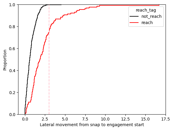
Immediately we can see that both curves do show some separation. For example,the first plot shows that using whether 3 feet of lateral movement between snap and engagement start, almost no “not reach” blocks would be accidentally classified as a reach block (as the black curve is almost at 1 on the y-axis at a value of 3). However, picking a value of 3 would miss a lot (~80%) of reach blocks, as around 80% of players moved less than 3 yards between snap and engagement.
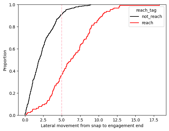
Looking at the second plot, which considers change from snap to the end of the engagement, we can see that the distinction between curves is larger. This indicates that this variable is likely a better option for our logic based approach. Here we can see that a cut off of 5 yards would correctly classify around 90% of the ‘not reach’ blocks and around 60% of reach blocks.
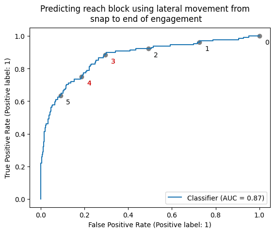
To help investigate this further, it can be helpful to plot this same data in a different way. Above, we have essentially been using the eCDF plots to examine the sensitivity, or true positive rate (probability of a given event being labeled reach block, given that we know it actually was a reach block on the field), using the red curve and specificity, or true negative rate (probability of labeled ‘not a reach’ block, given that we know it’s ‘not a reach’ block), using the black curve. We can also do this using ROC curves, which plot the true positive rate on the y axis and false positive rate (1 - true negative) on the x axis, for a range of different threshold values. As we want to minimize the false positive rate and maximize the true positive rate, thresholds closest to the top left of the plot are best. On the plot below, we label points which correspond to whole number cut offs. We can see that a threshold of 3 or 4 yards is suggested. A threshold of 3 would correctly identify more tagged reach blocks correctly (i.e. the true positive rate is higher than for a threshold of 4), but would also misclassify more ‘not reach’ blocks (i.e. the false positive rate is also higher). Due to where we expect this step of the logic to fit in the overall classification scheme, we decide on a cut off of 4 yards for this value.
Putting it all together
We’ve demonstrated how we put together our football knowledge and data with one example, looking at how to differentiate reach blocks with a single variable (lateral distance from snap to the end of the engagement). Of course, there are six more block types we need to identify as well, with many more variables to consider to help do this. We won’t go through the specifics for all the block types here, but we can follow a similar process to do this: starting with the building blocks (pun intended) put together by our SMEs and using data to help evaluate these further.
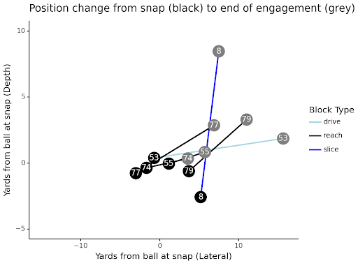
Here’s an example play, with the defined block type for each player indicated by the color of the line representing their post-snap movement. The plot shows the coordinates of the relevant players at the snap (black) and the end of the engagement (gray), in relation to the ball location at the snap. We can see that the reach blocks, shown by the black lines, all demonstrate a large amount of lateral movement. Although another block (number 53) also shows a large amount of movement, this is classified as a drive block. This is due to other layers of logic superseding the reach block assignment logic. A drive block is where the offensive player blocks a defensive player at an angle, with a good example being a down block on power.
Conclusion
When working with data, especially the extremely domain-specific data we have in this case, it’s important to take a collaborative approach between data scientists and SMEs. Although in this case we used a very logic-based approach, this also applies to research with more of a modeling focus. For example, discussions with SMEs can help identify additional features that may not otherwise be considered at the outset of a project, and confirm that final results align with their expectations once a model has been trained and tuned.
The main focus of this article has been to demonstrate how we developed our block-type logic. Keep an eye out for future articles that demonstrate how this data can be used to analyze players and teams.
