At StatsBomb, we pride ourselves on utilising the most cutting-edge technology to create better data. We have used Computer Vision (CV) in our event data collection since day one, relying on a combination of Human + Artificial Intelligence (AI) to provide the most accurate and detailed event data in the industry. Now, as we move into tracking data collection, we’re leveraging more and more AI to deliver highly accurate data at scale.
Last year, we published the first articles in our 'Creating Better Data' series from our AI team: Machine Learning Engineer Miguel Méndez Pérez explained what homography is and why it's important to our data collection, before Yohahn Ribeiro and Alex Palmer-Walsh explained how we use AI and Computer Vision technology to generate physical metrics. The latest article in this series comes from our Computer Vision Engineer Iñaki Rabanillo Viloria, who explains how exactly an engineer tasked with computing homography could go about calculating the homography of a given sports field or pitch - including example code so you too can calculate homography from still images.
Here's Iñaki.
1. Introduction
In this post, we will explain different approaches to compute the homography matrix that fully describes the transform between the 3D world and a 2D image of it. If you want some background reading on the subject, you can read this post on my github.
There are multiple ways to characterize the perspective transform. We will focus on estimating the homography matrix, as oposed to the more interpretable KRT parametrisation (focal length, rotation angles and 3D location).
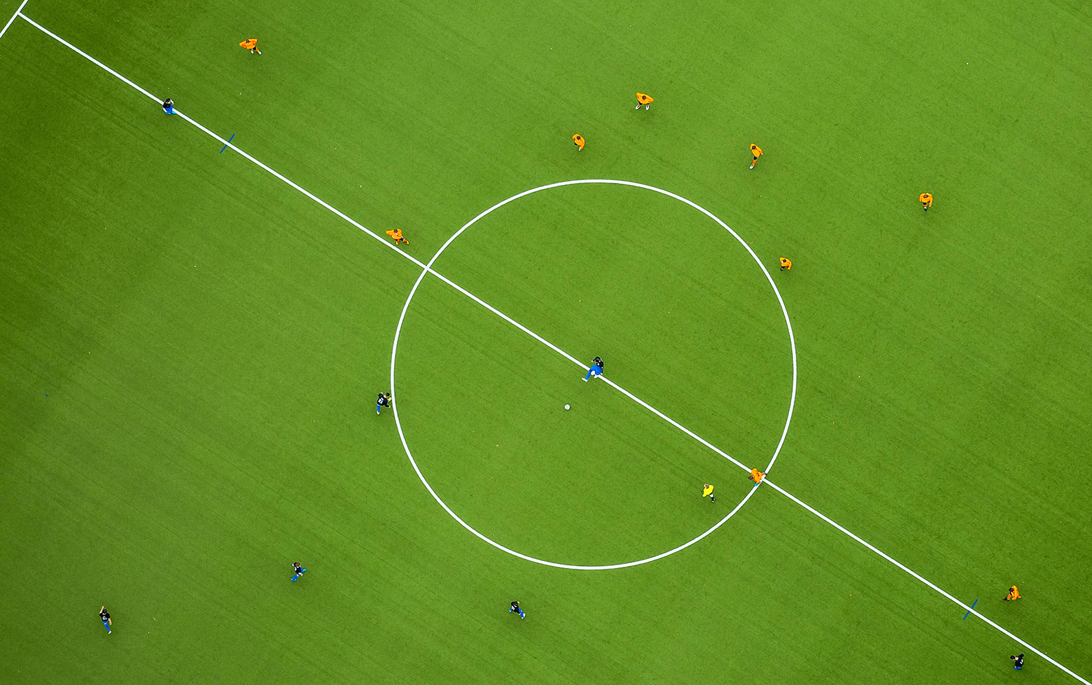
The reason for that choice is the implicit assumption that we are only given a 2D image to characterize the transform. Under that constraint, the KRT parametrisation is not resolvable, as illustrated in the image below. If we have a zenithal view of the pitch, we could end up capturing the exact same image by varying accordingly the distance to the ground and the focal length.
To resolve the ambiguity, we would need correspondences between points in the captured 2D image and non-coplanar points in the 3D world.
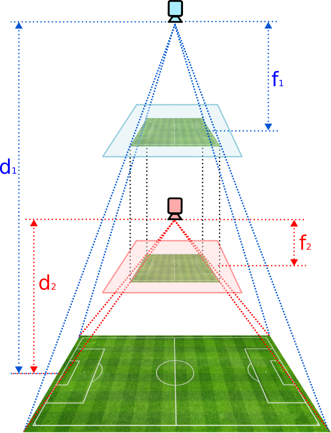
Figure 1. Depiction of a soccer field photographed by two different cameras from a zenithal view. By adjusting the focal length, it is possible to capture the exact same image of the field from both angles. This illustrates the ambiguity in trying to retrieve the camera parameters from a 2D image.
2. Geometric Features
We have explained in an earlier post how different types of geometric features \(g\) are mapped between the two domains via the homography matrix: \(g'=f_1(H, g)\). If we are able to identify corresponding features in both domains, we could then try to find a way to revert this process and compute \(H=f_2(g, g')\).
2.1. From points/lines
Let us start by the simplest scenario where all equations are linear. For the sake of simplicity, we will focus on the retrieval of the homography from a set of point correspondences. However, notice there is a duality between points \(\Longleftrightarrow\) lines.
$$
\begin{equation}
\vec{p'}=H\cdot\vec{p}
\end{equation}
$$
$$
\begin{equation}
\vec{l}=H^T\cdot\vec{l'}
\end{equation}
$$
As a result, the process of retrieving the homography from a set of line correspondences would be completely analogous.
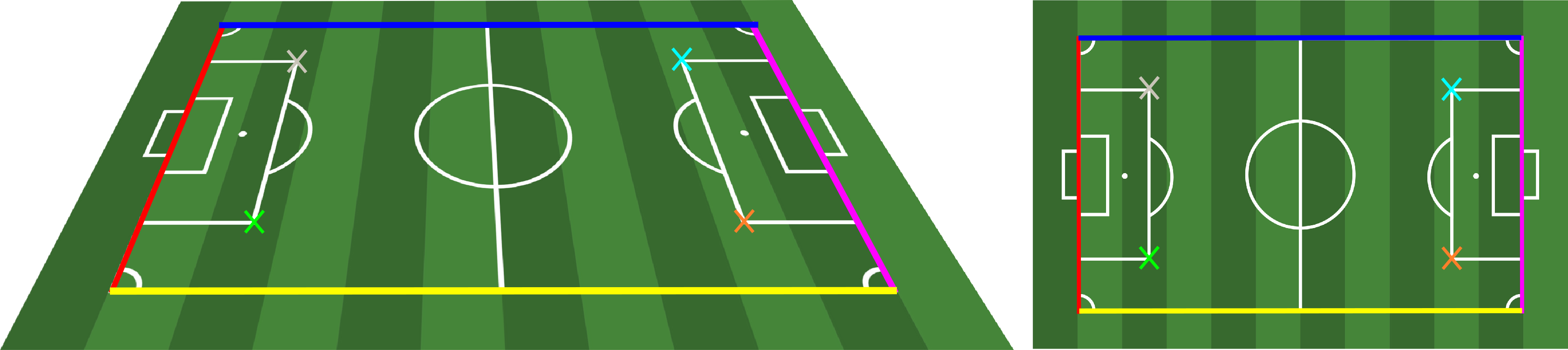
Figure 2. Example of non-collinear pairs of points and non-concurrent pairs of lines that would allow to retrieve the homography matrix
2.1.1. Problem formulation
We can expand the equation for projecting a point in homogenous coordinates between two 2D planes:
$$
\begin{equation}
s\cdot
\begin{bmatrix}
x' \\
y' \\
1 \\
\end{bmatrix}=
\begin{bmatrix}
h_{11} & h_{12} & h_{13}\\
h_{21} & h_{22} & h_{23}\\
h_{31} & h_{32} & h_{33}\\
\end{bmatrix} \cdot
\begin{bmatrix}
x \\
y \\
1 \\
\end{bmatrix}
\end{equation}
$$
For each homogenous coordinate, we get:
$$
\begin{equation}
s\cdot x'=h_{11}\cdot x + h_{12}\cdot y + h_{13}
\end{equation}
$$
$$
\begin{equation}
s\cdot y'=h_{21}\cdot x + h_{22}\cdot y + h_{23}
\end{equation}
$$
$$
\begin{equation}
s=h_{31}\cdot x + h_{32}\cdot y + h_{33}
\end{equation}
$$
By replacing \(s\) we arrive at:
$$
\begin{equation}
h_{31} \cdot x\cdot x' + h_{32}\cdot y \cdot x' + h_{33}\cdot x'=h_{11}\cdot x + h_{12}\cdot y + h_{33}
\end{equation}
$$
$$
\begin{equation}
h_{31} \cdot x\cdot y' + h_{32}\cdot y \cdot y' + h_{33}\cdot y'=h_{21}\cdot x + h_{22}\cdot y + h_{23}
\end{equation}
$$
We can vectorise the homography matrix elements into
$$
\begin{equation}
\vec{h}=\left[ h_{11}, h_{12}, h_{13}, h_{21}, h_{22}, h_{23}, h_{31}, h_{32}, h_{33}\right]^T
\end{equation}
$$
which gives us the following homogenous system:
$$
\begin{equation}
\begin{bmatrix}
x & y & 1 & 0 & 0 & 0 & -xx' & -yx'& -x'\\
0 & 0 & 0 & x & y & 1 & -xy' & -yy'& -y'
\end{bmatrix} \cdot
\vec{h} = 0
\end{equation}
$$
We can observe that a pair of points gives us two linear equations. Therefore, we could collect a set of point pairs and stack together all the equations to obtain a system of the form:
$$
\begin{equation}
A\cdot\vec{h}=0
\end{equation}
$$
2.1.2. Noise amplification: the horizon line
Importantly, this system is not very robust to noise corruption, and the contribution to the accuracy of the solution depends on the point location. To understand why, let us focus on the scenario depicted below.
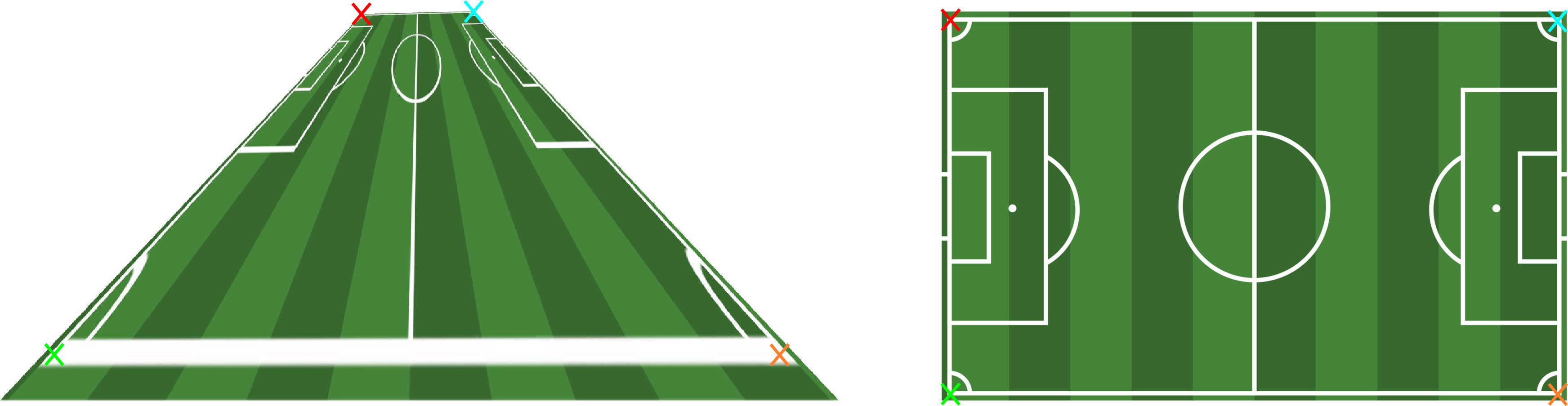
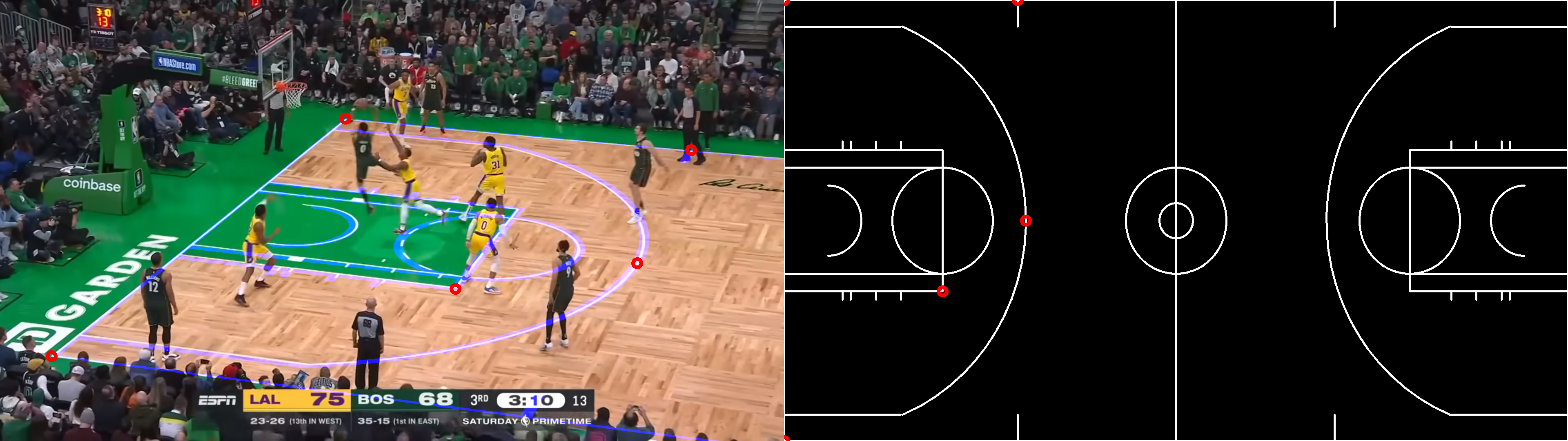
Figure 3. Example of 4 point pair correspondences.
We can observe that the upper sideline is relatively close to the horizon line. In the real world, the distance between its endpoints (red and cyan) is exactly the same as the distance for the bottom sideline endpoints (green and orange).
However, due to the perspective transform, that distance is substantially smaller in the projected space. When we label the pixel coordinates in the left image, a slight error in the points for the top sideline will correspond to a much bigger error in yards than an equivalent pixel error for the bottom sideline.
In order to mitigate the impact of deviations, a common strategy consists of labelling more than the minimum number of required points (four). In this way, we make our system more robust to noise contamination.
2.1.3. Solution: least squares estimator
The goal is thus to solve the homogenous system of linear equations of the form
$$
\begin{equation}
A\cdot\vec{h}=0
\end{equation}
$$
Recall that the matrix H has 8 degrees of freedom (DoF). In order to solve this system, we therefore need 8 linearly independent equations. This can be achieved by having 4 different and non-colinear points (or 4 different non-concurrent lines, equivalently).
If we have more points, the system will be overdetermined. In general, that means there will not be an exact solution, so it seems reasonable to instead solve the Total Least Squares (TLS) problem given by

We have added an extra constraint in order to avoid the trivial solution \(\vec{h}=\vec{0}\). Bear in mind that \(H\) is also only determined up to scale, so the unitary norm constraint is not restrictive at all (other constraints are also valid, such as \(h_{33} = 1\), which is also a common choice).
This problem can easily be solved by resorting to the Singular Value Decomposition (SVD) of matrix A
$$
\begin{equation}
A=U \cdot\Sigma \cdot V^T
\end{equation}
$$
where \(U\) and \(V\) are unitary matrices defining an orthonormal basis for the column and row space of \(A\) respectively. We can leverage this property for the following equalities
![]()

As a consequence, the system in \((13)\) is equivalent to

and if we redefine \(V^T\cdot\vec{h}=\vec{g}\), our problem has simplified substantially to

Since \(\Sigma\) is a diagonal matrix with its elements sorted in decreasing order

This sum is minimized by setting
$$
\begin{equation}
\vec{g}=\left[0, 0, \,\,\,\cdots\,\,\,, 0, 1\right]
\end{equation}
$$
Finally, recall that \(\vec{h}=V\cdot\vec{g}\), which implies that \(\vec{h}\) is just the eigenvector corresponding to the smallest eigenvalue.
On the other hand, if we just have four points or our observations are perfectly noiseless, the system \(A\cdot\vec{h}=0\) has a unique solution. In that scenario, \(A\) can be reduced to an \(8x9\) matrix of rank 8. That means it will have a 1D null-space from which we can compute a non-trivial (\(\vec{h}\neq \vec{0})\) solution: the eigenvector corresponding to the null eigenvalue.
Try it yourself!
You can see an example of how to retrieve the camera from a set of point/line correspondences in the repository. In order to do so, just install the package (`poetry install`) and then run
# from points
poetry run python -m sb_projective_geometry homography-from-point-correspondences-demo
# from lines
poetry run python -m sb_projective_geometry homography-from-point-correspondences-demo
This will generate the following figures:
OpenCV provides a built-in method that retrieves the homography from a set of point correspondences: cv2.findHomography()
You can try it out in the repo for comparison by calling:
camera = Camera.from_point_correspondences_cv2(pts_source=points_template, pts_target=points_frame)
2.2. From conics
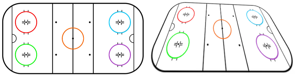
Figure 6. Example of conic correspondences found in a hockey ice rink template.
Similarly, we could try and estimate the homography from conic correspondences. We already know conics fulfill the following equation, up to a scale:
$$
\begin{equation}
s\cdot M'=H^{-T}\cdot M\cdot H^{-1}
\end{equation}
$$
where the scale factor satisfies
$$
\begin{equation}
s^3\cdot\text{det}(M')=\frac{\text{det}(M)}{\text{det}(H)^2}
\end{equation}
$$
We can freely force \(\text{det}(H)=1\), which implies:
$$
\begin{equation}
s=\sqrt[3]{\frac{\text{det}(M)}{\text{det}(M')}}
\end{equation}
$$
Therefore, without loss of generality, we can always normalize \(M'=s\cdot M\), so \(\text{det}(M)=\text{det}(M')\) and get rid of the scaling factor.
Under the assumption that the conics are non-degenerate (\(\text{det}(M)\neq 0)\), we can combine this equation for two pair of corresponding ellipses \(\{(M_i, M_i'),\,\, (M_j, M_j')\}\)
$$
\begin{equation}
M_i^{-1}\cdot M_j=H^{-1}\cdot M_i'^{-1}\cdot M_j'\cdot H
\end{equation}
$$
or equivalently
$$
\begin{equation}
H\cdot M_i^{-1}\cdot M_j-M_i'^{-1}\cdot M_j'\cdot H = 0
\end{equation}
$$
This forms a set of linear equations in the elements composing the homography matrix \(H\). Consequently, we can form a system of equations similar to the one we resolved earlier:
$$
\begin{equation}
B_{ij}\cdot\vec{h}=0
\end{equation}
$$
Importantly, two pairs of ellipses are not enough to uniequivocally determine the homography. We instead need at least 3 pairs of ellipses. By stacking the equations correspondinh to each combination of two pairs of ellipses, we arrive at the final system
$$
\begin{equation}
B\cdot\vec{h}=0
\end{equation}
$$
that we can solve following the procedure defined for the previous scenario.
Try it yourself!
You can see an example of how to retrieve the camera from a set of ellipse correspondences in the repository. In order to do so, just install the package (`poetry install`) and then run
# from ellipses
poetry run python -m sb_projective_geometry homography-from-ellipse-correspondences-demo
This will generate the following figure:
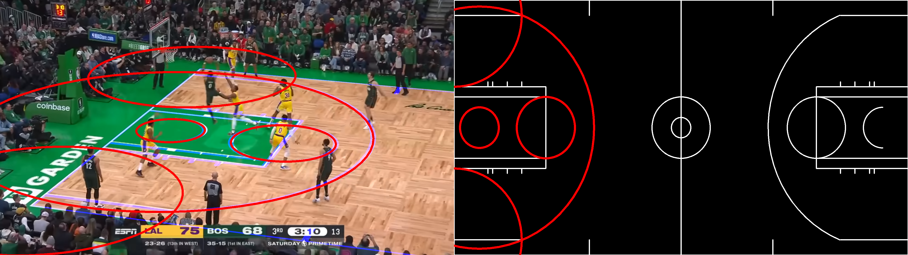
Figure 7. Retrieve homography from annotated ellipses (red). Pitch template projection from retrieved homography is displayed in blue.
2.3. From multiple features
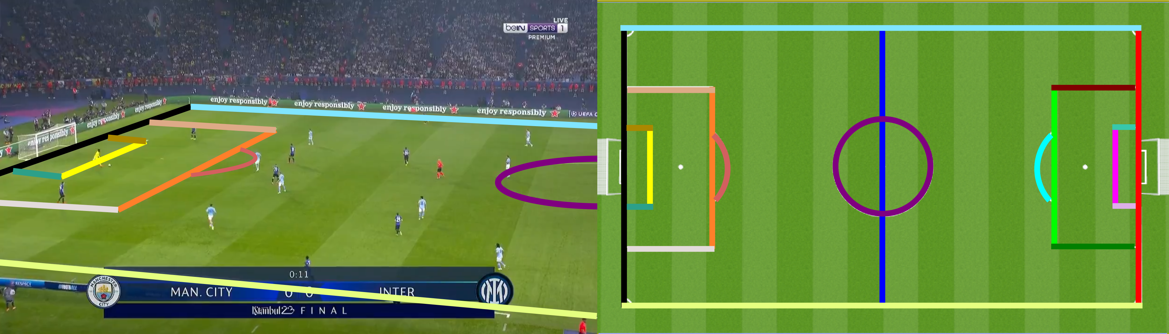
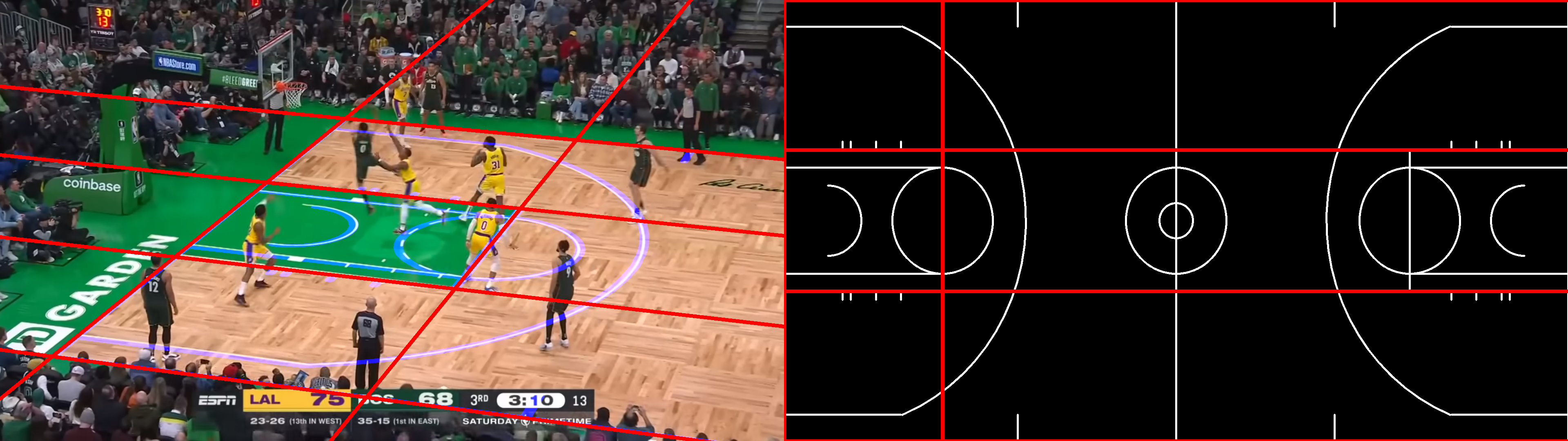
Figure 8. Example of different types of geometric features correspondences between a football broadcast frame and the pitch template.
If we have identified a set of different matching geometric features (i.e.: points, lines, conics), one could solve the problem by trying to minimize a cost function that combines multiple terms. Ideally, one should be able to compute a convex metric that captures the similarity for each type of feature.

Figure 9. Example of distances (marked in green) between pairs of (a) points, (b) lines and (c) ellipses.
This way, finding the homography boils down to solving the following optimisation problem

Try it yourself!
You can see an example of how to retrieve the camera from a set of point, line and ellipse correspondences in the repository. In order to do so, just install the package (`poetry install`) and then run
# from ellipses
poetry run python -m sb_projective_geometry homography-from-correspondences-demo
This will generate the following figure:
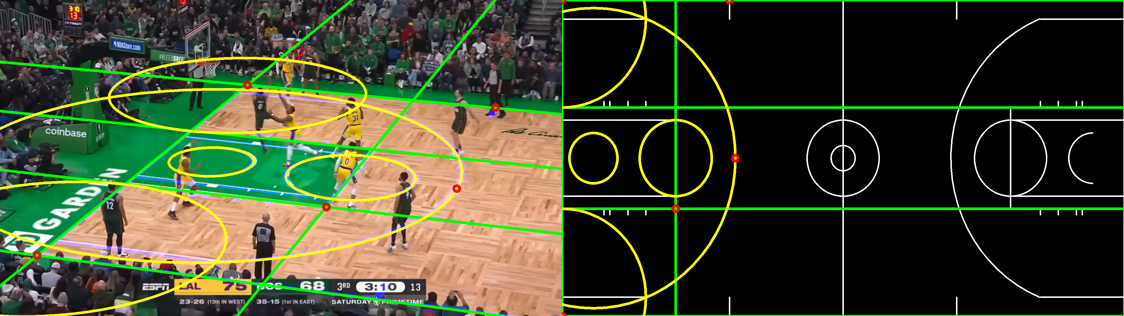
Figure 10. Retrieve homography from annotated points (red), lines (green) and ellipses (yellow). Pitch template projection from retrieved homography is displayed in blue.
3. Via a pair images
So far we have focused in retrieving the homography from a set of matching geometric features. What if instead we are given two photographs of the same scene taken from different angles?

Figure 11. Two photographs of the Eiffel Tower taken from different angles.
One way to proceed would be to identify and match geometric features, then apply the previously described procedures. The identification could be done manually, or automatically. The latter has been an active area of research over recent decades, and multiple methods can be used, such as Harris corner detector, Canny edge detector, SIFT features, SURF features or ORB features. Interestingly, some of these detectors serve as descriptors too, which in turn provides a way to pair them out of the box.
Alternatively, one could view the homography estimation as a registration problem. Let us say we have two images, the source \(I(\vec{x})\) and the target \(T(\vec{x})\), where \(\vec{x}=[x, y]^T\) corresponds to the pixel coordinates for the images. Moreover, let \(W(\vec{x}; \vec{h}) = H\cdot \vec{p}\) be the transform that warps a set of pixels under the projective transform. \(H\) would be the homography matrix characterizing the transform, and \(\vec{h}\) its vectorized form. Then we can minimize the following cost function:
$$
\begin{equation}
\sum_{\vec{x}} |I(W(\vec{x}; \vec{h})) - T(\vec{x}) |^2
\end{equation}
$$
Lucas-Kanade (LK) is a popular iterative algorithm widely used to tackle this kind of problem [6]. It relies on the computation of the gradient, under the assumption that objects may be located at different positions across the two images, but their appearance remains the same. There are multiple extensions, such as:
- Hierarchical LK: resolves the problem at multiple resolutions to estimate iteratively gross-to-fine motion.
- Multimodal LK: for images where contrast varies (such as in between CT-scans and MRIs), but structure remains. Thus, the pixel intensity similarity is not a valid metric anymore. Instead, metrics based on entropy or sparisty can be used (see [7] for details).
Given a set of geometric features identified in one of the images, LK algorithm can also be used directly to solve the matching step. However, it is important to rely on static features. If moving objects are used instead, that would corrupt the estimation of the camera motion.
Try it yourself!
You can see an example of how to retrieve the camera from two images in the repository. In order to do so, just install the package (`poetry install`) and then run
# from images
poetry run python -m sb_projective_geometry homography-from-image-registration
This will grab the following two images:

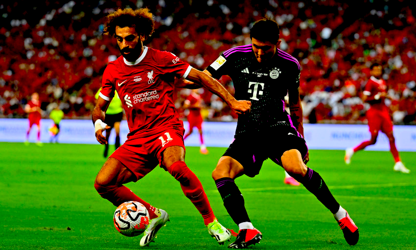
It will try to find a set of matching keypoints in both, as illustrated below:
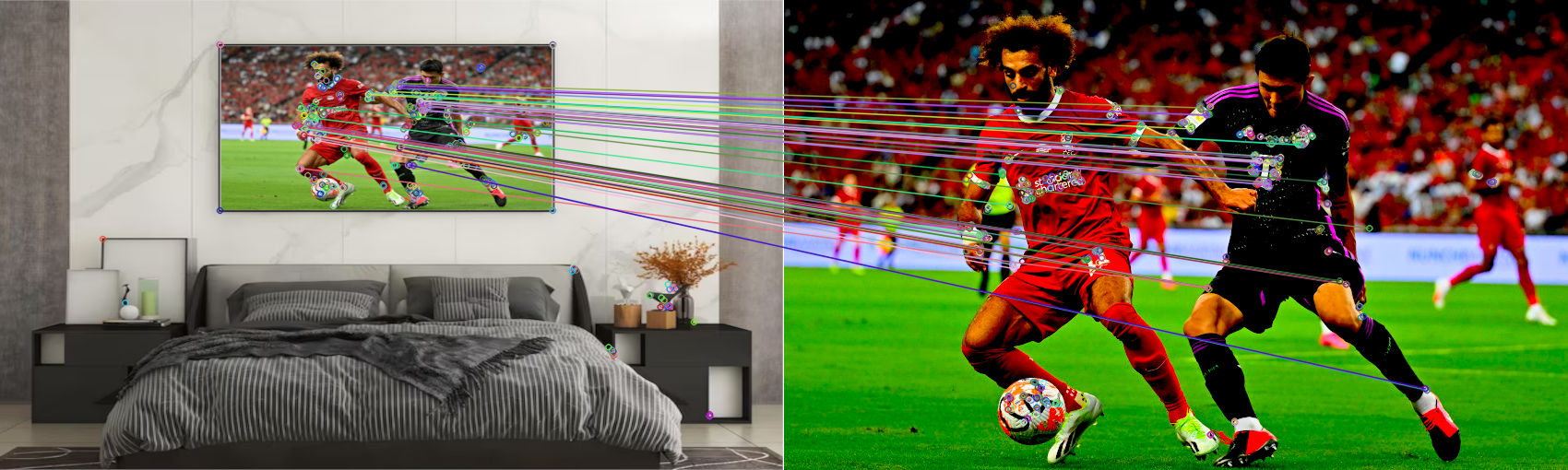
Figure 14. Set of identified matching keypoints.
And it will use those to retrieve the homography that allows to warp the source image (red border) onto the target one:

Figure 15. Source image (red border) warped onto the target image with the retrieved homography..
4. Via ML model
Finally, a modern approach to tackle the homography estimation problem consists of using an ML trained model that is able to predict the projective transform given the input. If we’re trying to align two given images, those would serve as the input to the model. Alternatively, if we’re trying to map a given image to pre-defined template, one would only need to provide the former, since the template is static. For the sake of simplicity, we will focus on this second case.
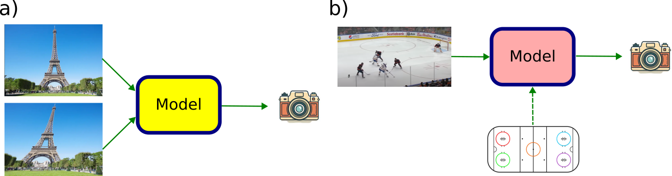
Figure 16. a) Model that predicts the projective transform parametrisation that aligns two given images, b) Model that predicts the projective transform parametrisation that aligns a given image against a pre-defined static template.
One feature that seems to have a substantial impact in the quality of the predictions is the parametrisation used to characterize the projective transform. The possible choices are:
- Homography matrix: the model would directly regress the parameters in the homography matrix. However, as pointed out in [8], those parameters consist of a mix of both rotational, translational and shearing terms. Therefore, they will likely vary in very different scales, so it would be necessary to balance their contribution to the loss.
- Projected geometric features: alternatively one could parametrize the homography by the projected coordinates of a set of pre-defined geometric features. In the simplest case, it would suffice to use 4 points, as proposed in [8, 9]. Alternatively, in order to increase the robustness in the prediction, one could create a grid of \(N\times M\) points and predict the locations for all of them. Moreover, one could also predict other features such as lines, ellipses… as done in [11].
From the two set of geometric features (the pre-defined static one, and its projected version predicted by the model), it would suffice to apply one of the procedures described before in order to retrieve the homography matrix.
For the sake of the explanation, let us say we choose to predict the location of the projection for a set of points within a rectangular grid. Another important choice is therefore what domain to predict their location in. There are two choices here:
1. Template domain: this forces the model to implicitly learn the mechanics of the projective transform, since it will have to learn their location after projecting the image grid to the template domain (see below).
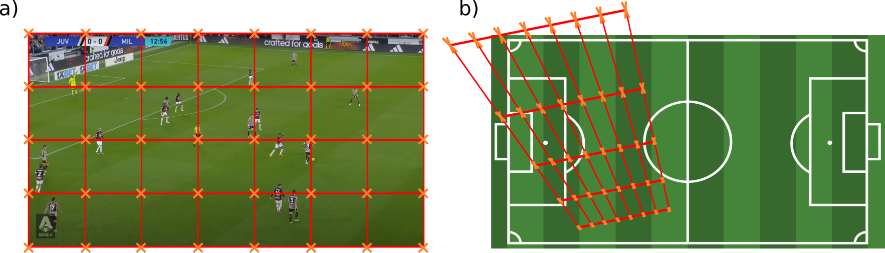
Figure 17. a) Static grid in image domain whose projection the model will have to learn, b) Projected grid predicted by the model for the given frame.
The hope is that the model, by means of ingesting enough data, is able to learn these mechanics. However, it seems very inefficient to ask the model to learn this transform when its characterization is already known and mathematically described. Therefore, the following approach seems a much better way to tackle the problem.
2. Image domain: this alleviates the complexity of the task at hand, since the model will only have to learn to identify the relevant keypoints in the given image.
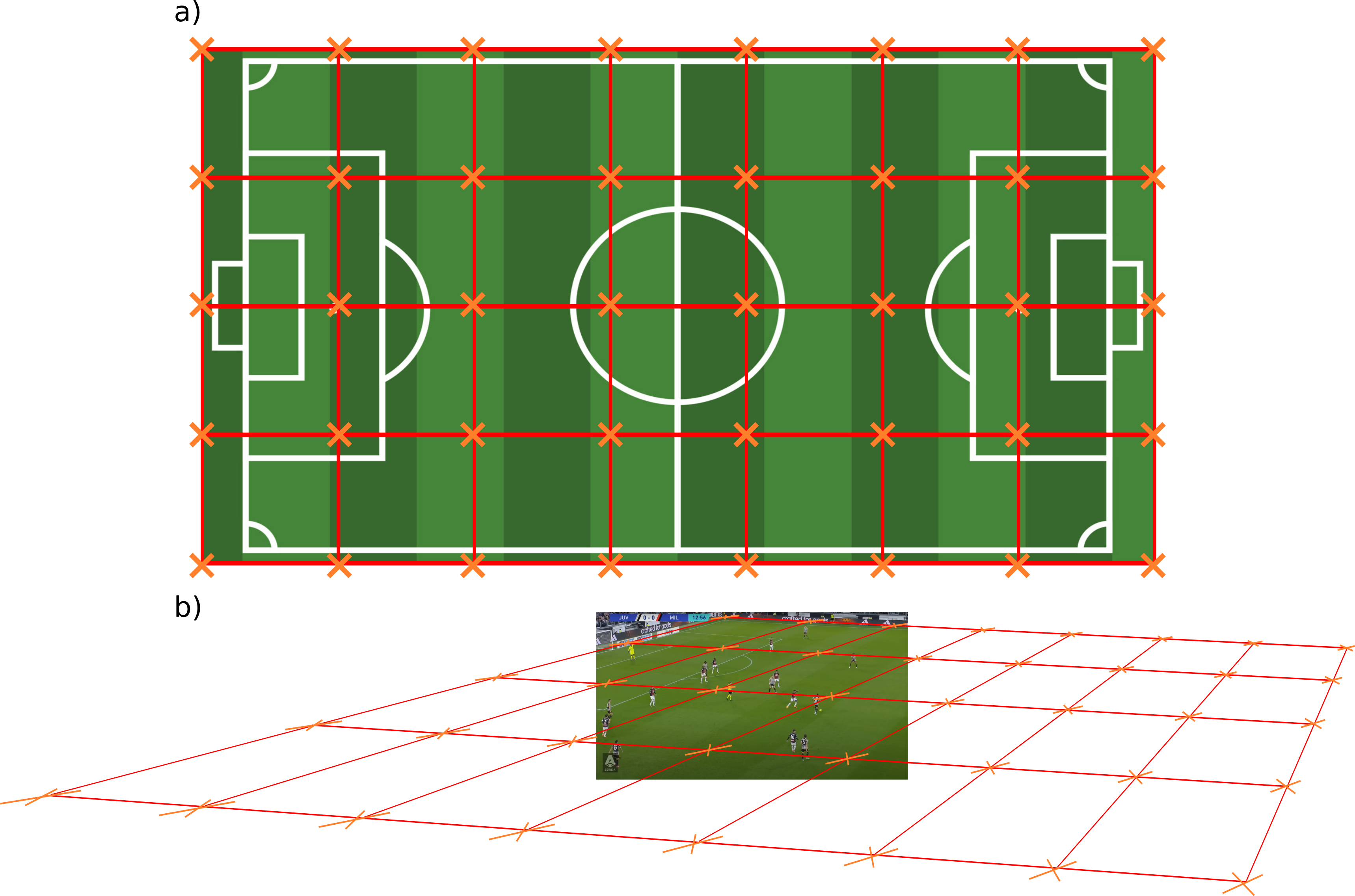
Figure 18. a) Static grid in template domain whose back-projection the model will have to learn, b) Back-projected grid predicted by the model for the given frame.
As we have stated, by using a grid with more than the bare minimum required (4 points), we make the process more robust to noise corruption. However, this comes at a cost: the model is now free to predict the keypoints in a way that does not correspond to a projective deformation of a rectangular grid.
Once again, the expectation is that, with enough data, the model will implicitly learn there is a relationship between the keypoints in the grid. But asking the model to learn that well-known relationship seems an inefficient usage of the available data. So there is a trade-off there between robustness and data efficiency.
On the other hand, predicting the features location allows for another in choice. The problem can be posed as:
- Regression problem: in this case, one would simply train the model to predict the x-y coordinates of the geometric feature in question, resorting to any regression loss such as the l2 distance.
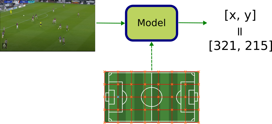
Figure 19. Model is asked to find pixel (x-y) coordinates of selected template keypoint (marked in cyan) in the given image.
- Classification problem: alternatively, one could train the model to predict the probability of each pixel in the image corresponding to the sought-out keypoint, and then estimate its location by taking the one with the highest one.
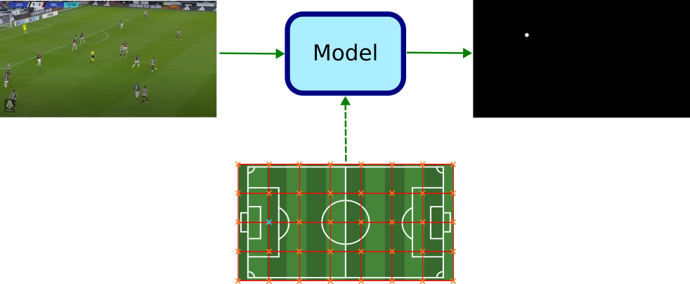
Figure 20. Model is asked to predict the probability (color-coded in grayscale) of a pixel in the given image to correspond to selected template keypoint (marked in cyan)
Why bother to solve a regression problem via classification instead? Well, although this is not yet well-understood, there is empirical evidence pointing towards classification being more accurate at the regression task. The following Twitter thread provides some insights of why that might be the case.
ML theory twitter, here is a question: why classification works so much better that regression?
Bonus question: is it true only for DL, or for XGBoost as well? https://t.co/YEM45JBjhZ— Dmytro Mishkin 🇺🇦 (@ducha_aiki) November 1, 2022
One hypothesis revolves around the gradient computation during training. [12] argues that regression loss results in a smaller gradient the closer we get to the correct output. On the other hand, the gradient for the classification loss does not depend on how close we are to the underlying true value. This means that for bad predictions, the first loss is able to correct faster. However, once the prediction enters the small error regime, the classification approach would be more effective at narrowing the gap to the ground-truth.
Another hypothesis suggests that when dealing with multi-modal data, whereas regression forces the model to make a choice, classification allows it to express uncertainty. In our case, the model could express that by assigning similar probability scores to multiple disjoint areas in the image. In such a way, the model may therefore be able to better capture the underlying multi-modal distribution of the input.
Summary
In this post we have shown multiple approaches that allow to retrieve the homography matrix. Those include:
- Techniques that rely on manual input, i.e. labelled geometric features such as keypoints, lines or ellipses.
- Techniques exploiting classical computer vision algorithms, such as Lukas-Kanade.
- Techniques based on Deep Learning models
The latter constitute the state-of-the-art and is illustrated in the video below. It displays the pitch template (red) projected using the homography retrieved in a fully automated fashion.
6. References
[1] Richard Hartley and Andrew Zisserman (2000), Multiple View Geometry in Computer Vision, Cambridge University Press.
[2] Henri P. Gavin (2017), CEE 629 Lecture Notes. System Identification Duke University, Total Least Squares
[3] Richard Szeliski (2010), Computer Vision: Algorithms and Applications, Springer
[4] OpenCV Libary: Basic concepts of the homography explained with code
[5] Juho Kannala et. al. (2006), Algorithms for Computing a Planar Homography from Conics in Correspondence, Proceedings of the British Machine Vision Conference 2006.
[6] Simon Baker and Iain Matthews (2004), Lucas-Kanade 20 years on: A unifying framework. International Journal of Computer Vision.
[7] Lucilio Cordero Grande et. al. (2013), Groupwise Elastic Registration by a New Sparsity-Promoting Metric: Application to the Alignment of Cardiac Magnetic Resonance Perfusion Images, IEEE Transactions on Pattern Analysis and Machine Intelligence.
[8] Detone et.al. (2016), Deep Image Homography Estimation, arXiv.
[9] Ty Nguyen et. al. (2018), Unsupervised Deep Homography: A Fast and Robust Homography Estimation Model, arXiv.
[10] Wei Jiang et. al. (2019), Optimizing Through Learned Errors for Accurate Sports Field Registration, 2020 IEEE Winter Conference on Applications of Computer Vision (WACV)
[11] Xiaohan Nie et. al. (2021), A Robust and Efficient Framework for Sports-Field Registration, 2021 IEEE Winter Conference on Applications of Computer Vision (WACV)
[12] James McCaffrey (2013), Why You Should Use Cross-Entropy Error Instead Of Classification Error Or Mean Squared Error For Neural Network Classifier Training
[13] Iñaki Rabanillo (2023): Projective Geometry: Building the Homography Matrix from scratch
[14] Iñaki Rabanillo (2023): Projective Geometry: Projecting between domains
