“Pressure” occurs when one or more defensive players start to track down the QB, causing the QB to get rid of the ball or attempt to scramble or move in the pocket to avoid getting sacked. Previously at StatsBomb, our pressure counts have been derived from a range of variables regarding defender proximity to the QB and their involvement in engagements with blockers. While we believe this initial approach gave a good overall metric for pressures, we can generate additional insights using a model-based approach. Here we’ll briefly outline that in-progress model and provide a sneak peek at some of the results.
Although we are interested in evaluating pressures, we chose to train our model using sacks. In essence, sacks are the most extreme form of pressure, and we’d expect similar features in our data to be associated with both sacks and pressures. Sacks are also much easier to define. Ask multiple analysts if a sack occurs on a play and you’d likely get the same answer, but judgements as to when a pressure occurs would be much more variable. The comparative consistency of sacks makes this a better choice as a model target, as otherwise the model could have difficulty learning the relationships between the features and the target (if multiple analysts tag the data in slightly different ways), or be geared towards one specific definition of a pressure which may not align with other analysts (if one analyst tags all the data).
Based on our prior experience using a logic-based approach to determine pressures, as well as other published work evaluating line play (most notably, 2023 NFL Big Data Bowl submissions), we already had a good idea about which features would be needed for the model.
Unsurprisingly, the most important feature to the model is distance between the defensive player and the QB. Other important features include:
- The speed at which this distance has changed compared to previous frames
- The “engagement status” of the defensive player (players in an engagement are less likely to generate a pressure)
- A feature to differentiate between NFL and NCAA games. This allows the model to better pick up the relationships that are similar across NFL and NCAA (e.g. smaller distance between QB and defender -> higher probability of sack), while also accounting for any differences. A similar approach has also been used in our EPA and CPOE models.
The model is trained using data from every tracking frame in each passing play, with the play ending in a sack or not as the target variable. The model can thus evaluate the likelihood of a sack at any given time point in the play. This means we can see how the likelihood of a sack develops over a play in a way that we can’t using a simpler heuristic approach. The output of the model is the probability of a sack occurring on the play, given the features from the current frame, where 1 means that the model is 100% certain a sack will happen and a value of 0.5 means the model believes a sack will occur on this play around half the time.
Laiatu Latu
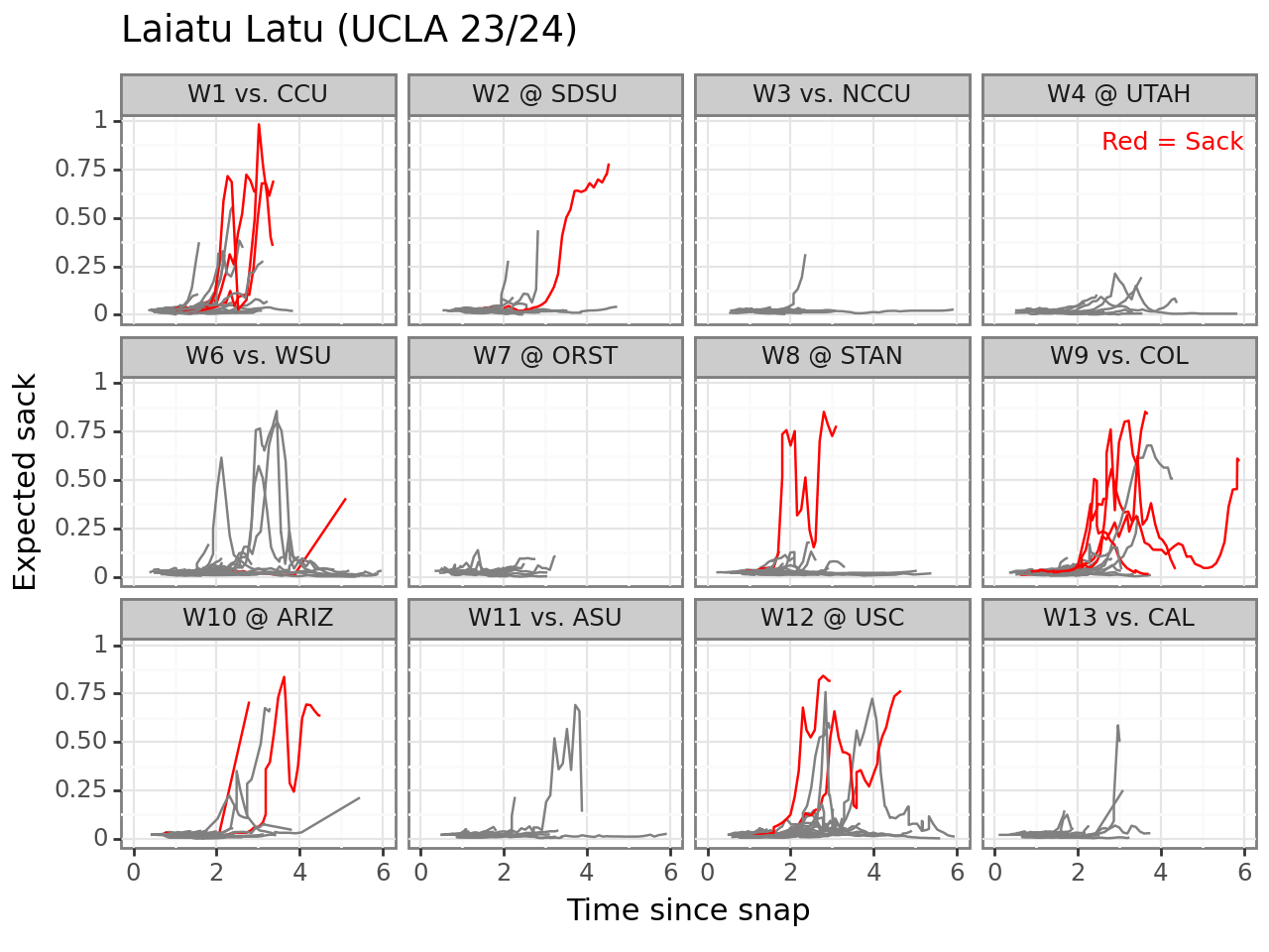
To see how this works in practice, let’s take a look at all the games Colts’ first round pick Laiatu Latu played for UCLA last season. This visualization shows each game as a separate panel, with time since snap on the x-axis and expected sack (the output of our model) on the y-axis. Plays where Latu sacked the QB are highlighted in red. This provides an overall snapshot of Latu’s performance across the season, with respect to both how often he generates pressure and when in the play this occurs.
There are some games where he generates very little pressure (e.g. against Oregon State in week 7) and others where the pressure is significantly higher (e.g. against Coastal Carolina in week 1).
Of course, the expected sack metric alone doesn’t tell the full story. The actions of the QB can make a huge difference to whether a sack occurs - multiple studies have demonstrated sacks allowed are a QB stat as much as an offensive line metric. A given QB might tend to release passes early, or move to evade the pressure, while others are more likely to hold the ball and remain stationary. If the QB always releases the ball early, there is unlikely to be much opportunity for the defender to create pressure.
In the UCLA games we are considering for this analysis, the average time to pass from snap ranges between 2 and 3 seconds. However, the QB throws the ball within a second on some plays and holds it for over 7 seconds on others.
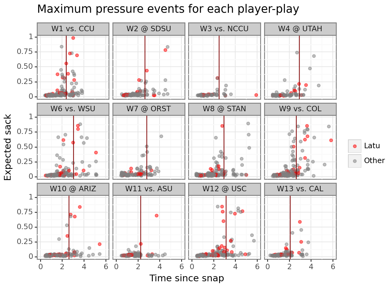
To evaluate the relationship between the time the QB holds the ball and the amount of pressure generated, we can look at the maximum expected sack value for each defensive player on each play. Essentially this means we are looking at the point in time where each defensive player generates the most pressure. We plot the time of the maximum pressure event for each player-play combination on the x-axis and the expected sack value for that event on the y-axis. The vertical lines show the average time to pass/sack for each game. Although there are high pressure events occurring early on some plays, there is a correlation between longer plays and higher pressure events.
We can also view individual plays in a similar way. Below, we can analyze the pressure generated over a play resulting in a sack by Gary Smith III. In this example, we can see that numerous defensive players generated some level of pressure on the QB well before the sack occurred. So while Smith was credited with the sack, our expected sack metric allows us to evaluate the impact of other defenders as well. The relatively high values for expected sack for players who did not record a sack on the play is a good indication that our model has utility for evaluating pressures as well as sacks.

So far we have looked at expected sacks independently of the outcome of the play. But the aim of creating pressure is to force poor decisions by the QB and limit the amount of yards/first downs gained.
Below we plot the maximum expected sack from any defensive UCLA player on each play against the number of yards gained on the play (including both air yards and yards after catch, where applicable). We see that, as expected, higher pressure is correlated with fewer yards gained on the play. However, it seems like this may largely be driven by sacks resulting in a loss of yards. It should be noted that this analysis only includes passing plays- therefore plays where the QB scrambles and gets past the line of scrimmage are not included. Deriving inference for plays where the QB scrambles will be incorporated as part of the final stage of model development.
Next steps
In this analysis, we have focused on how pressure develops over the course of a play, by deriving the probability of a sack occurring over the course of a play. However, there are many alternative ways we could consider this- for example, we may want to look at plays where pressure is maintained over a given threshold for a set period of time (e.g. expected sack > 0.4 for at least a second). One of the next steps of our development work will be to evaluate different methods of utilizing the model to see which best captures the characteristics of a pressure which produces results which generally concur with expert observers’ criteria for “pressures”. This will also include expanding our inference to include plays where the QB scrambles.
