
We are five matchdays into the season in La Liga, so let’s have a look at some emerging trends from the early action. Spain Remains Light on Shots La Liga saw the least shots, goals and expected goals (xG) of any big five European league last season, and things have been even tighter in the early running of the new campaign. All three measures are down. While the English, Italian and German top flights have each averaged over three non-penalty goals per match, Spain has averaged just two, right in line with xG. There have been three less shots per match (20.30) than in any of the other leagues. Even in the context of a competition that remains steadfastly low on goalmouth action, Athletic Club stand out as a particularly bad watch. Their matches to date have barely averaged over a single expected goal and have featured the lowest shot count (15.25) of any in the league. A Promising Start for Betis Real Betis always looked like one of the prime candidates to move up the table this season. Their 15th place finish last time around was allied to top eight metrics, and the attacking talent within the squad is such that even a minor defensive improvement, whether through luck or judgement, was always going to make them top eight contenders. Nine points from their first five matches under Manuel Pellegrini represents a good start and has them second in the nascent table, albeit with at least two or three teams behind who will probably better their points haul once games in hand have been played. Even with defeats to Real Madrid and Getafe thrown into the mix, Betis have begun the campaign as a shot dominant team, outshooting their opponents in all of their matches and taking 64% of the total shots across those fixtures. It is a good starting point, but the difference between the quality of shots taken and conceded means they still have a negative expected goal difference at this stage. They are taking a few too many speculative efforts in attack... 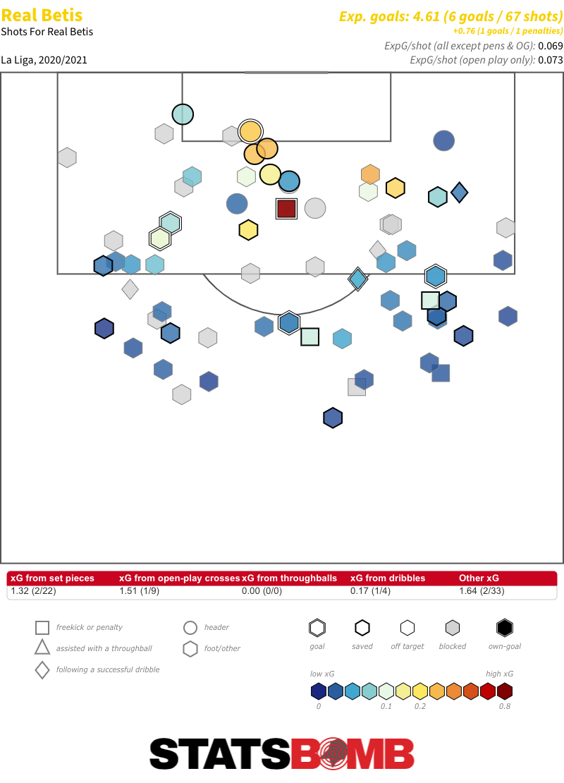 ...and while their higher defensive line and slightly more aggressive off-ball approach has so far done a solid job of suppressing opposition shot volume, the chances they have conceded have generally been high-quality ones.
 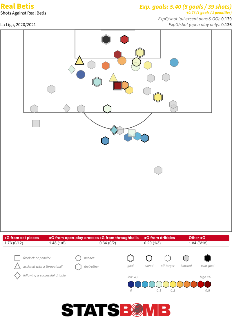 With that said, they have already played Real Madrid, which skews things in such a small sample size. It is also unlikely those shot quality numbers will hold throughout the campaign given that they would have been comfortably the worst in La Liga at both ends of the pitch last season. As things begin to equalise out a bit, we’ll have a better idea if Betis are genuine European contenders. Underpowered Elche Elche have only played three times to date, and do already have four points on the board, but they’ve looked decidedly underpowered on their return to the top flight following a five-year absence. Unsurprisingly so, given that they weren’t even a standout side in the Segunda División last season. They made it up through the playoffs after finishing sixth in the table with bottom six metrics. Add to that a new head coach and the ridiculously short period of time they had to prepare for the top flight due to the delayed promotion playoffs, and it is to be expected that they've looked out of their depth. Jorge Almirón’s side have averaged a pitiful four shots per match while conceding more than 18. They were outshot 27 to five by Real Sociedad in their opener, and then 18 to two by fellow newly promoted side Huesca in a 0-0 draw prior to the international break.
 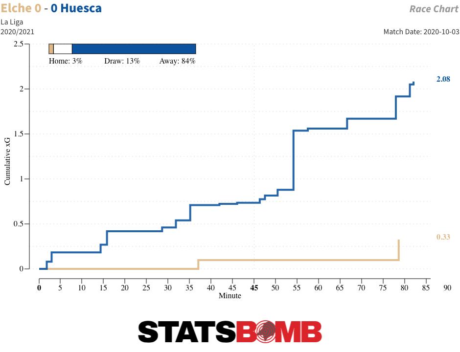 The squad has been reinforced with a flurry of late deals, no one can take the points they’ve already got away from them, and their shot numbers will naturally smooth out a little over time. But performances will have to improve massively if Elche are to have any chance of remaining in the division. New Arrivals Doing Their Thing David Silva may only have started three of Real Sociedad’s five matches to date, but he still leads the league in total open play passes into the penalty area. On a per-90 basis, he ranked in the top four of the Premier League in that metric for Manchester City in each of the last four seasons, and it seems he will again be amongst the most prolific suppliers in La Liga.
 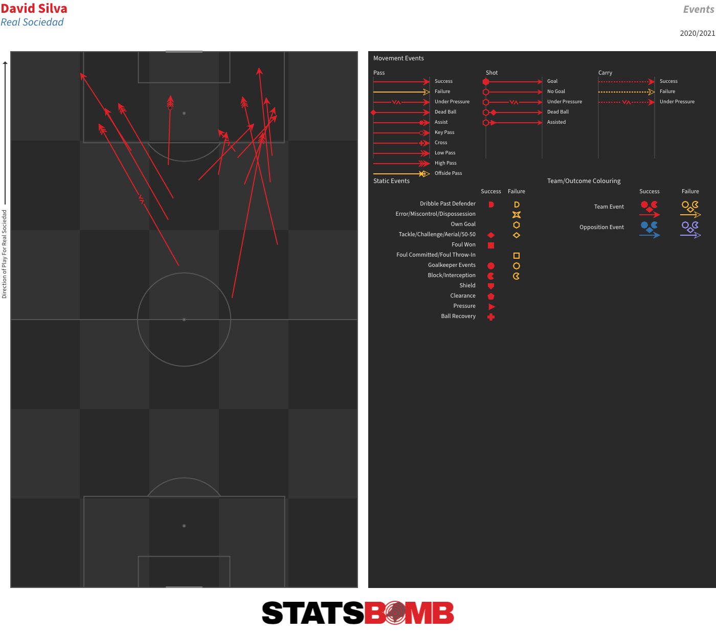 Dani Parejo may not have any goals or assists to his name since his off-season move from Valencia to Villarreal, but he’s continued to be the same reliable ball progresser as always.
 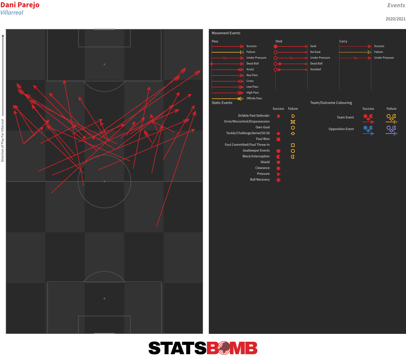 Emre Mor is back at Celta Vigo, and even if he hasn't done much else, he continues to be a prolific dribbler.
 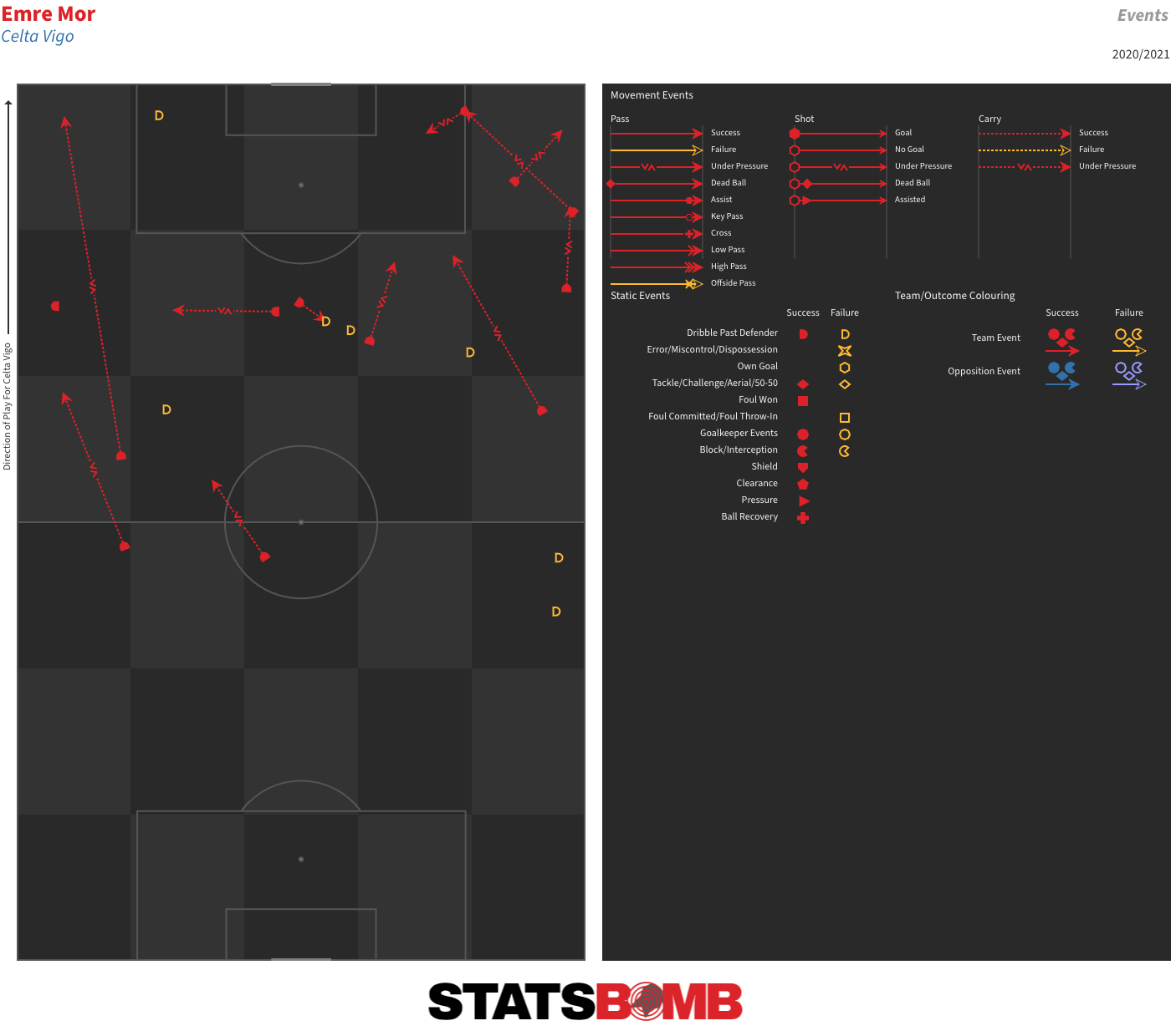 And Javi Ontiveros may have only seen a combined 90 minutes or so of action for Huesca after joining on loan from Villarreal, but the player who last season took more shots per 90 amongst players who saw at least 900 minutes of action than anyone but Lionel Messi has already got off four efforts on goal -- just below his 2019-20 average.
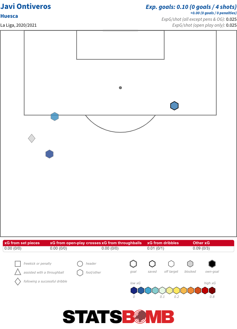
Ligue 1 was the first of the big five European leagues to get its 2020-21 season underway. Five matchdays in, let’s look at four interesting things from the early running in France. Rennes Lead The Way Rennes are the early leaders after taking four wins and a draw from their opening set of fixtures. Their underlying numbers also look promising, continuing the trend from the second half of last season’s abruptly shortened championship, when they had the second best metrics in the division behind Paris Saint-Germain. Then, a switch to a more proactive defensive approach, albeit still a pretty average one in the overall context of the league, yielded dividends at both ends of the pitch. Rennes began to create a higher number of better quality shots whilst conceding a lower number of worse quality ones. They became much more adept at creating opportunities in transitional phases of play, and leaned less on crosses as a means of entering the penalty area. 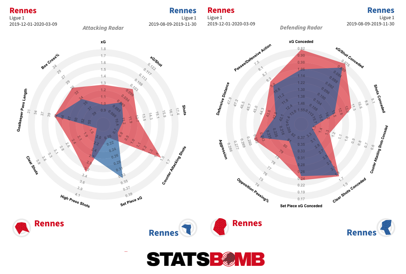 Those same broad stylistic traits seem to have carried into the early running of 2020-21, and their position atop the table is reflective of a smart club seemingly on the up. They won the Coupe de France in 2018-19, and last season’s third-place finish means that this time around they will compete in the Champions League for the first time in their history. Paris Saint-Germain: Still Good Paris Saint-Germain started the season poorly with consecutive 1-0 defeats to Lens and Marseille, a pair of results that predictably produced rumblings over the future of head coach Thomas Tuchel and talks of potential dressing room unrest. They’ve since recorded three straight wins without conceding, and their metrics suggest all is well. PSG have taken 66% of the shots in their matches and accumulated nearly 73% of the expected goals. They were genuinely bad against Lens in their opener, mainly because they were missing a bunch of key players including Ángel Di Maria, Kylian Mbappé, Marquinhos and Neymar, but they’ve otherwise been their normal dominant selves. As much as everyone would love to see a tighter title race, there is scant evidence of any kind of downturn or easing on their part. Even if a team like Lille, Lyon, Marseille, Monaco or Rennes does improve significantly, PSG were so insanely far ahead of the rest last season that even a slight easing in their output would still likely make them comfortable champions. A Great Start for Lens Newly promoted Lens have so far not looked at all out of place in the top flight. Three wins and a draw from their first five fixtures have them up in the top six, and their metrics look even better. They’ve taken a 63% share of the shots in their matches, and have carried an xG difference of +6.43 through these early weeks of the campaign, second only to PSG. Realistically, they aren’t going to maintain those numbers through the entire season, but it is a great start, and there is much to like in their approach. The new arrivals also seem to be producing. Gaël Kakuta is enjoying himself as one of two attacking midfielders in their 3-4-2-1 system, while Ignatius Ganago already has four goals (from 3.75 xG) on the board. Facundo Medina has replicated the bold ball-carrying and impressive passing range that saw him stand out at Talleres de Córdoba last season.
 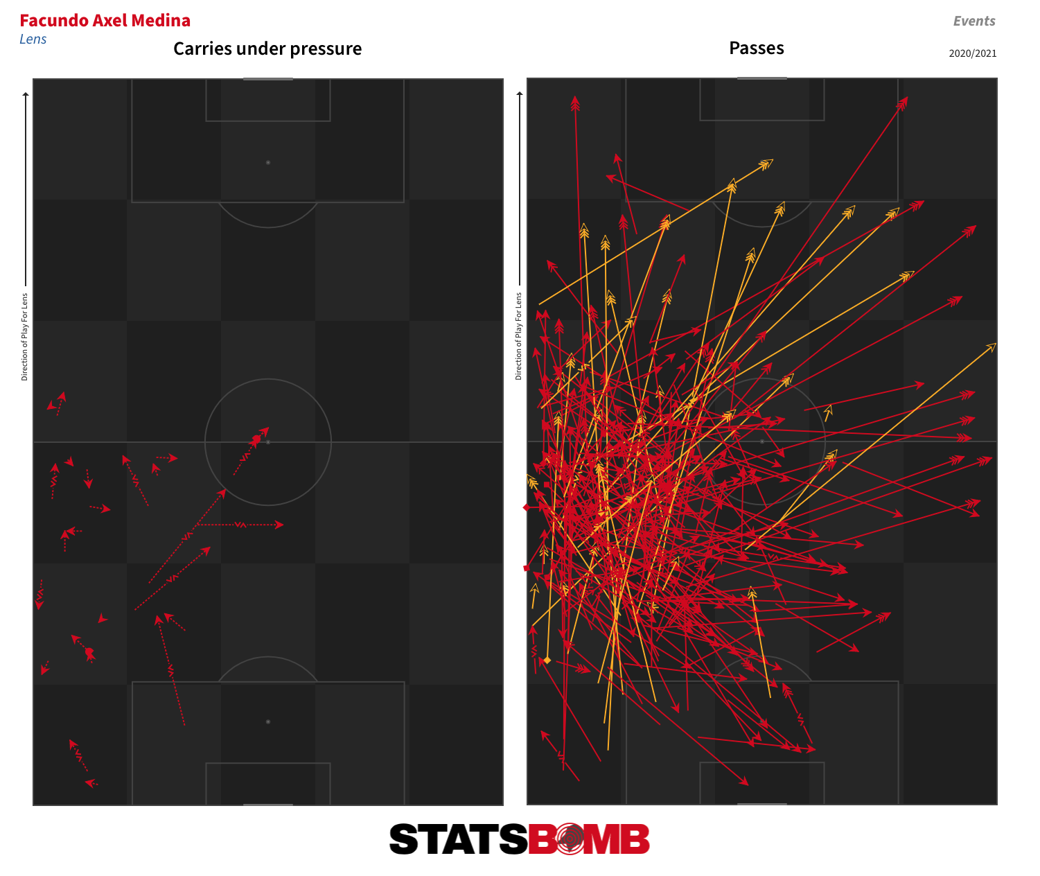 The underlying numbers also suggest that Lorient, who came up ahead of Lens as Ligue 2 champions, have been better than results to date might indicate. The two promoted teams have avoided a direct return to the second tier in each of the last two Ligue 1 seasons. That run might just continue through 2020-21. Bamba Finally Gets His Goal After 12 non-penalty goals in 2018-19, Lille’s Jonathan Bamba failed to register a single goal from 44 shots last season -- the highest non-scoring tally in the league.
 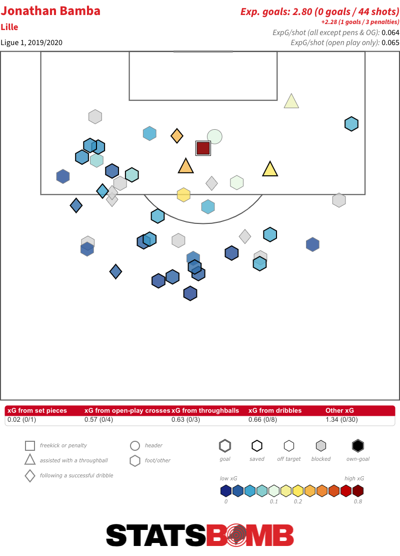 There was a bit of finishing variance involved there, but there was also a notable decline in the value of his shot locations in a post-Nicolas-Pépé world. The average quality reduced from 0.11 xG/shot in 2018-19 down to 0.06 xG/shot in 2019-20. But things seem to be looking up for Bamba this time around. He scored with his first shot of the new campaign in the opening day draw against Rennes, and added another in the 1-0 win away at Reims that followed it.
 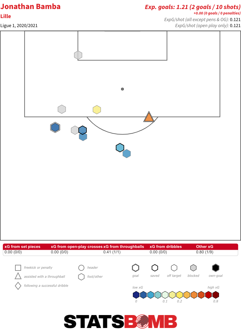 Lille have rebuilt their attack again this year following the big-money departure of Victor Osimhen to Napoli, and the changes seem to be to Bamba’s liking. The sample size is way too low to extrapolate too much from it, but the early signs are promising for a return to his output of two seasons past.
One of the advantages of using data in the early stages of a scouting process is the ability to filter down to a list of interesting players in a given role. It’s been a while since we’ve done some straight up data scouting on the site, so let’s try and identify some players aged 21 or under who stand out in the numbers in terms of creative passing and chance creation.
This article is also avaliable in Spanish.
Our search will include all the top flight leagues in our database as well as the second divisions of England, France, Germany, Italy and Spain. It will also only include players who have seen at least 1,200 minutes of action during the 2019-20 season (or 2019 or 2020 for those leagues that operate on a calendar-year basis). The given ages are how old the players would have been at the end of this season, had it completed on time.
The three metrics we’ll filter by are open play expected assists, open play passes into the box and throughballs. To whittle things down, we’ll look for players who are roughly inside the top 50 in the age group in all three. That produces the following cutoffs:
- 0.16 open play expected assists per 90
- 1.35 open play passes into the box per 90
- 0.22 throughballs per 90
We’ll also apply a filter on the percentage of successful box entries achieved by crosses in an attempt to weed some of the more classic winger types.
That gets us down to these 11 players.
| Name | Team | Age | Minutes | Throughballs | Open Play Passes Into Box | Open Play xG Assisted |
|---|---|---|---|---|---|---|
| Calvin Stengs | AZ Alkmaar | 21 | 2276.00 | 0.75 | 2.89 | 0.32 |
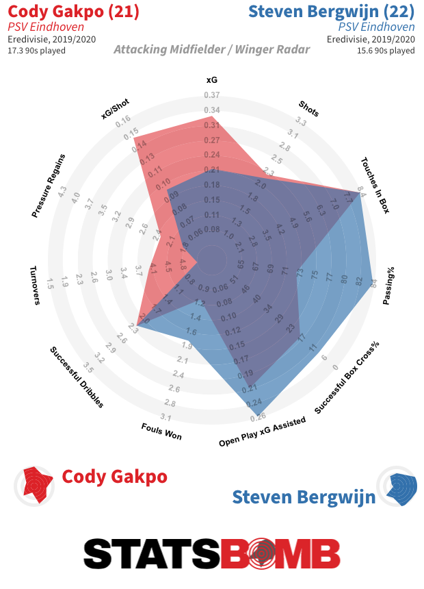
| Cody Gakpo | PSV Eindhoven | 21 | 1553.08 | 0.29 | 1.62 | 0.23 |
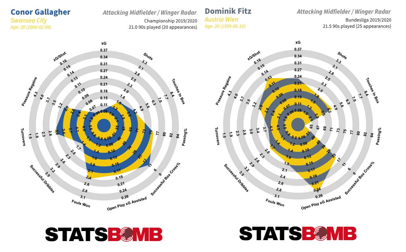
| Conor Gallagher | Swansea City | 20 | 1891.27 | 0.24 | 1.38 | 0.17 |
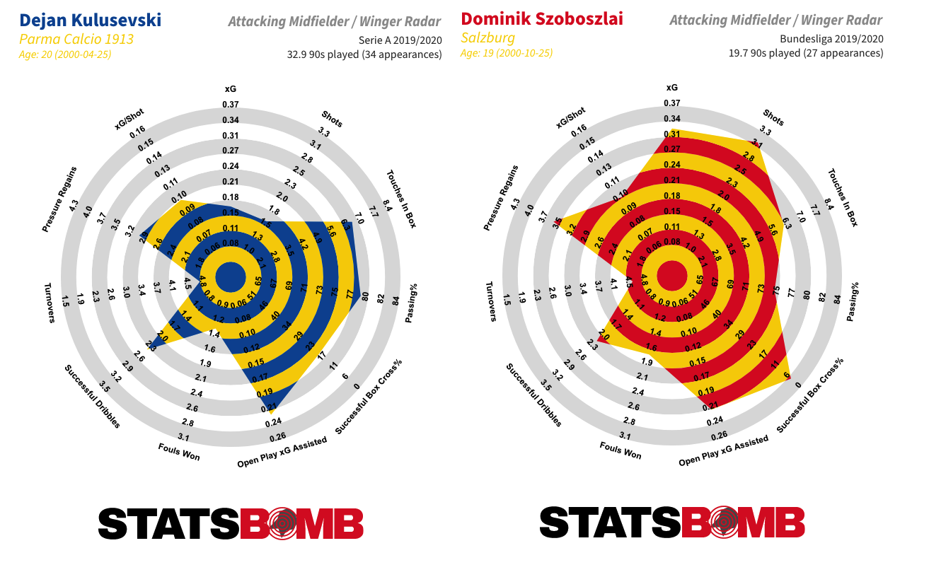
| Dejan Kulusevski | Parma Calcio 1913 | 20 | 2959.12 | 0.24 | 1.37 | 0.22 |
| Dominik Fitz | Austria Wien | 20 | 1937.52 | 0.51 | 2.18 | 0.25 |
| Dominik Szoboszlai | Salzburg | 19 | 1771.57 | 0.46 | 1.68 | 0.23 |
| Jadon Sancho | Borussia Dortmund | 20 | 2388.43 | 0.38 | 2.19 | 0.30 |
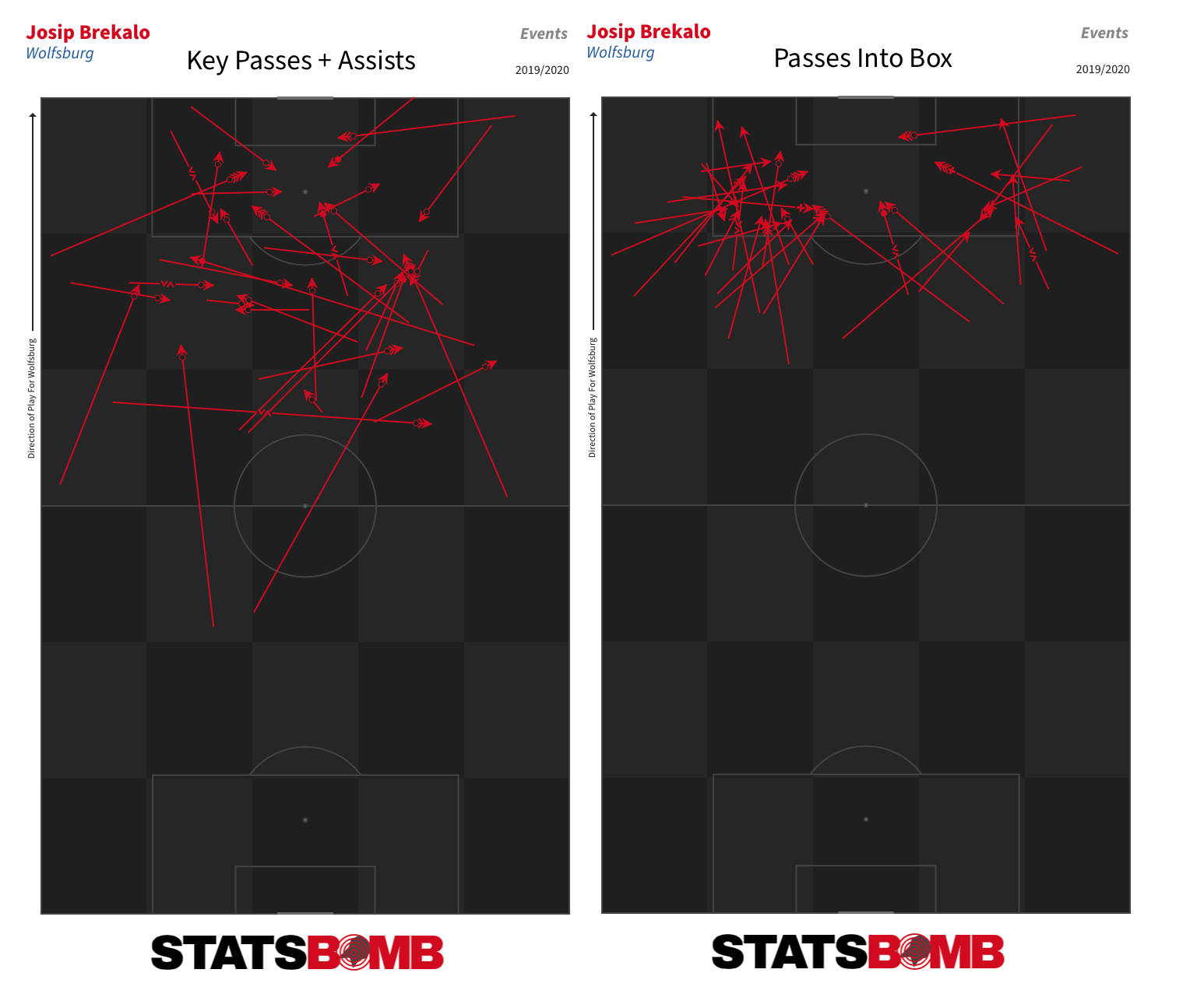
| Josip Brekalo | Wolfsburg | 21 | 1771.28 | 0.56 | 1.73 | 0.24 |
| Krepin Diatta | Club Brugge | 21 | 1778.28 | 0.40 | 2.08 | 0.17 |
| Kylian Mbappé | Paris Saint-Germain | 21 | 1620.90 | 0.22 | 1.44 | 0.48 |
| Nikola Čumić | Radnički Niš | 21 | 1825.20 | 0.35 | 1.58 | 0.25 |
That looks like a promising list. We’ve got Jadon Sancho and Kylian Mbappe, the two outstanding attacking talents in the age group. In January, Juventus paid €35 million for Dejan Kulusevski before loaning him back to Parma for the rest of the season. Dominik Szoboszlai is a part of the successful Red Bull ecosystem and there seems to be interest from Arsenal and Milan.
Running the same search for the 2017-18 and 2018-19 seasons spits out names like Christopher Nkunku, João Félix, Martin Ødegaard, Malcom, Steven Bergwijn and Mbappe again, so it seems like we are on the right track.
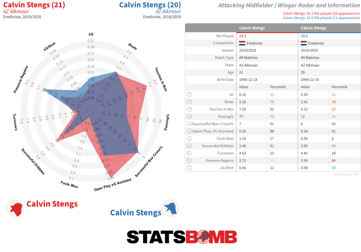
Another player who appears in both this season and last season’s list is Calvin Stengs. He’s a player I’ve always liked the look of, so it’s nice to see him here. He was also featured in our Pro Scouting product.
Stengs is a throughball machine, and the majority of the chances he creates begin and end in central areas. Of the players on the list, only Mbappe and Nikola Čumić create a better average quality of chance.
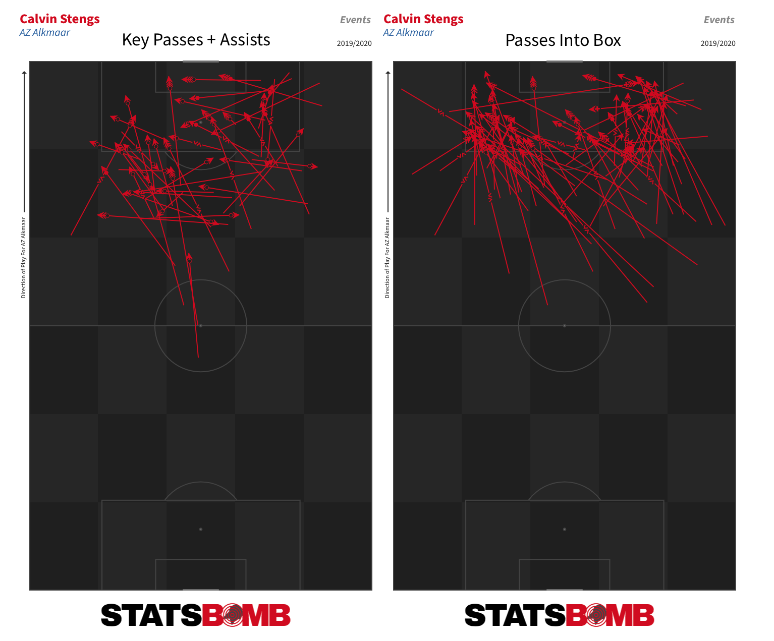
He also appears to be improving season on season, suggesting he could be ready to make a step up.
Nikola Čumić looks a good all-round attacking talent, or at least he has in the fairly weak Serbian League.

While his aptitude for moving the ball into the penalty area and creating chances appears to partly be due to his ability to create space off the dribble, something that might not carry to a stronger league, there is a decent variety in his passing in advanced areas.
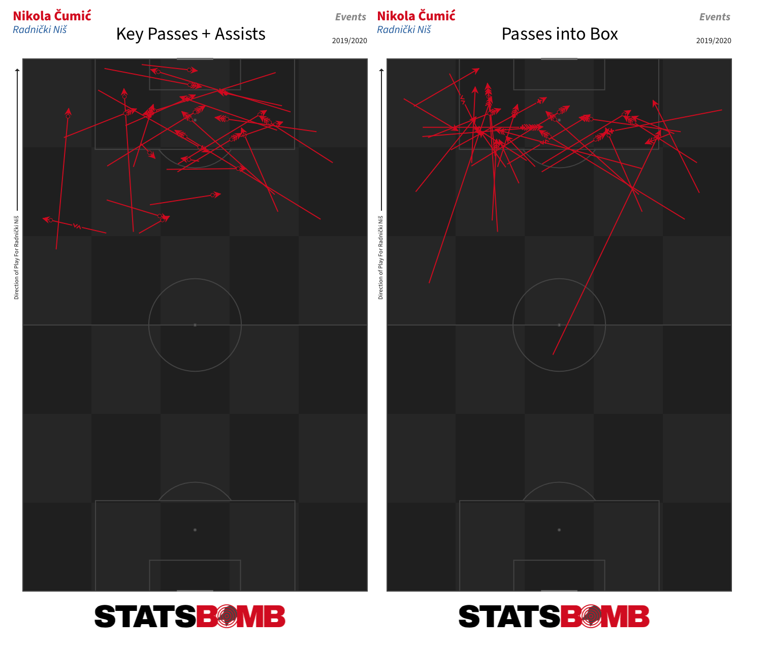
That kind of output from a young player rarely goes unnoticed. Olympiakos signed up Čumić in December before loaning him back to Radnički Niš until the end of the campaign. If he plays in European competition with the Greek champions next season, we might get a better idea of his level.
From the limited footage I’ve seen of him, Krepin Diatta looks an intriguing little player. At Club Brugge, he has played at right wing-back, with a few stints on the right and left flanks. But with Senegal he’s sometimes played in central midfield, where his incisive passing, dribbling and ball-carrying ability also look a good fit. There is a little bit of a lower-budget Tanguy Ndombele about him there, and it would be interesting to see him get a run in that role at club level.
Cody Gakpo became a regular starter for PSV Eindhoven following Bergwijn’s departure to Tottenham Hotspur in January. He has done a more than decent job of approximating his output.
There are things to like about all these players. Conor Gallagher, on loan at Swansea from Chelsea, and Dominik Fitz see more of the ball in deeper areas than the others and aren’t anywhere near as active on the dribble, but combine good creative numbers with solid defensive output.
Josip Brekalo is second in the Bundesliga in throughballs per 90, and seems to be pretty adept at working the ball into the penalty area when he cuts in off the left.
That is one of the interesting things about creating this kind of list: you find that players with similar output in one facet of play can have wildly differing overall profiles. That is one of the reasons why any competent club would carry out thorough qualitative scouting of these players before deciding whether to move for any of them. Data should play a key role in any modern recruitment process, but it is always just one element of many.

Four months after a ball was last kicked, Liga MX returns on Thursday for the first half of the 2020-21 season, which will carry the name of the Torneo Guard1anes in honour of the effort and sacrifice of healthcare workers during the COVID-19 pandemic in Mexico. Here are some teams, players and trends that stand out in the data as ones to keep an eye on. This article is also available in Spanish. Over and Under-Performing Teams 2019-20 Apertura champions Monterrey performed terribly in the Clausura prior to its premature end in March. They had lost five and drawn five and were yet to record a victory. But the underlying numbers suggest there was little to be unduly concerned about. Antonio Mohamed’s team found themselves in the rather unique situation of combining the league’s best non-penalty expected goal (xG) difference with its worst non-penalty goal difference. 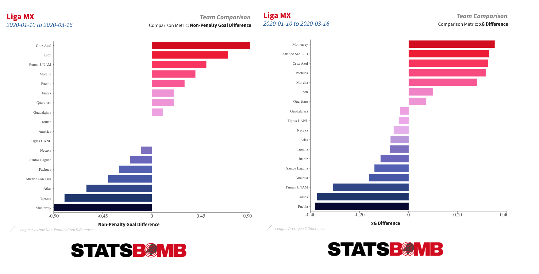 Over time, those kinds of things tend to even themselves out, and that is just as true the other way around. Over the full course of the 2019-20 season, no team outperformed their xG difference to the extent that Necaxa did, but even they started to drift back towards their underlying numbers during the Clausura.
 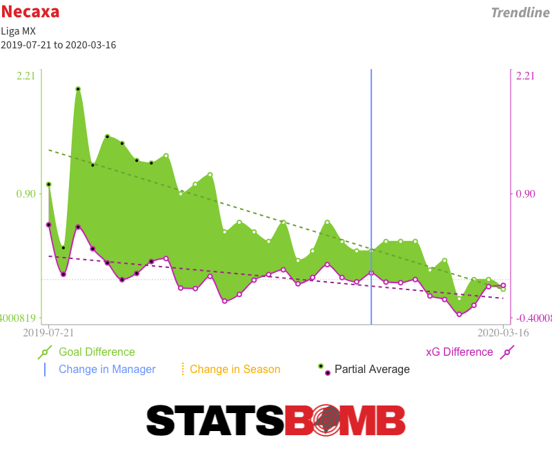 That should be of concern to teams like Puebla and Pumas. Both were in the playoff hunt during the aborted Clausura but had some of the league’s worst underlying numbers. León: The Throughball Masters On an outright basis, León had the best attack in Liga MX last season, and their expected goals tally was also up there with the league’s best. Yet their attack functioned very differently to those of the other high-scoring teams. They took a below league-average number of shots, but their average chance quality was far and away the best in the division.
 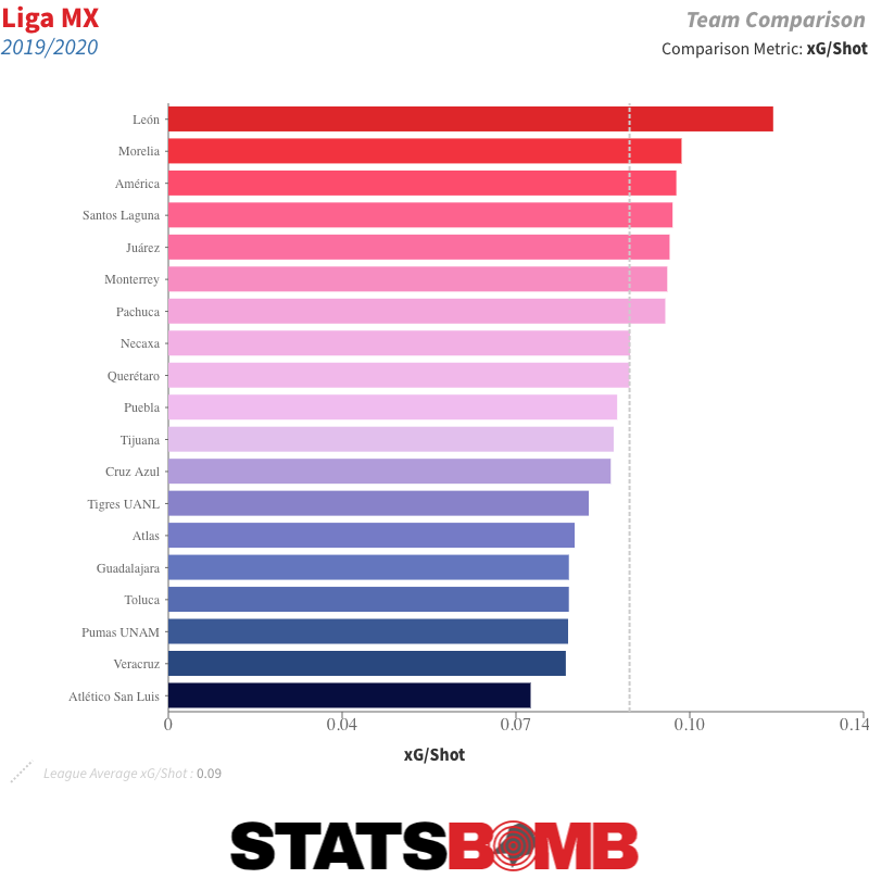 A look at their shot map provides us with a good idea as to why. See all those triangles? Those are shots from throughballs.
  Let’s separate them out.
  That is a lot of throughball shots -- 11 more than any other side, and almost twice as many on a proportional basis. Over 20% of León’s xG and goals came from them. Throughballs produce some of the highest quality chances in the game, and León create a ton of them. On an individual basis, the league’s top two throughball providers and four of the top five play for Léon: Luis Montes, Joel Campbell, Fernando Navarro and Pedro Aquino. You’ll also find Ángel Mena and Leonardo Ramos inside the top 15. So if you like yourself a good throughball, León are clearly the team to watch. On the opposite end of the scale, Chivas were the only team not to score a single goal from a throughball last season. Lopsided Attacks Last week, we had a look at the most lopsided attacks across the major European leagues, and the same general trends we saw there hold in Liga MX. Teams take a marginally higher percentage of their shots, generate a marginally higher percentage of their xG and score a marginally higher percentage of their goals from the left than the right. As in the major European leagues, shots from the centre account for around 75% of the goals. In the 2019-20 season, Puebla were the team with the biggest swing to one side in terms of the proportion of shots from the left and right that were taken from each side. They took 59.42% of those shots from the left:
 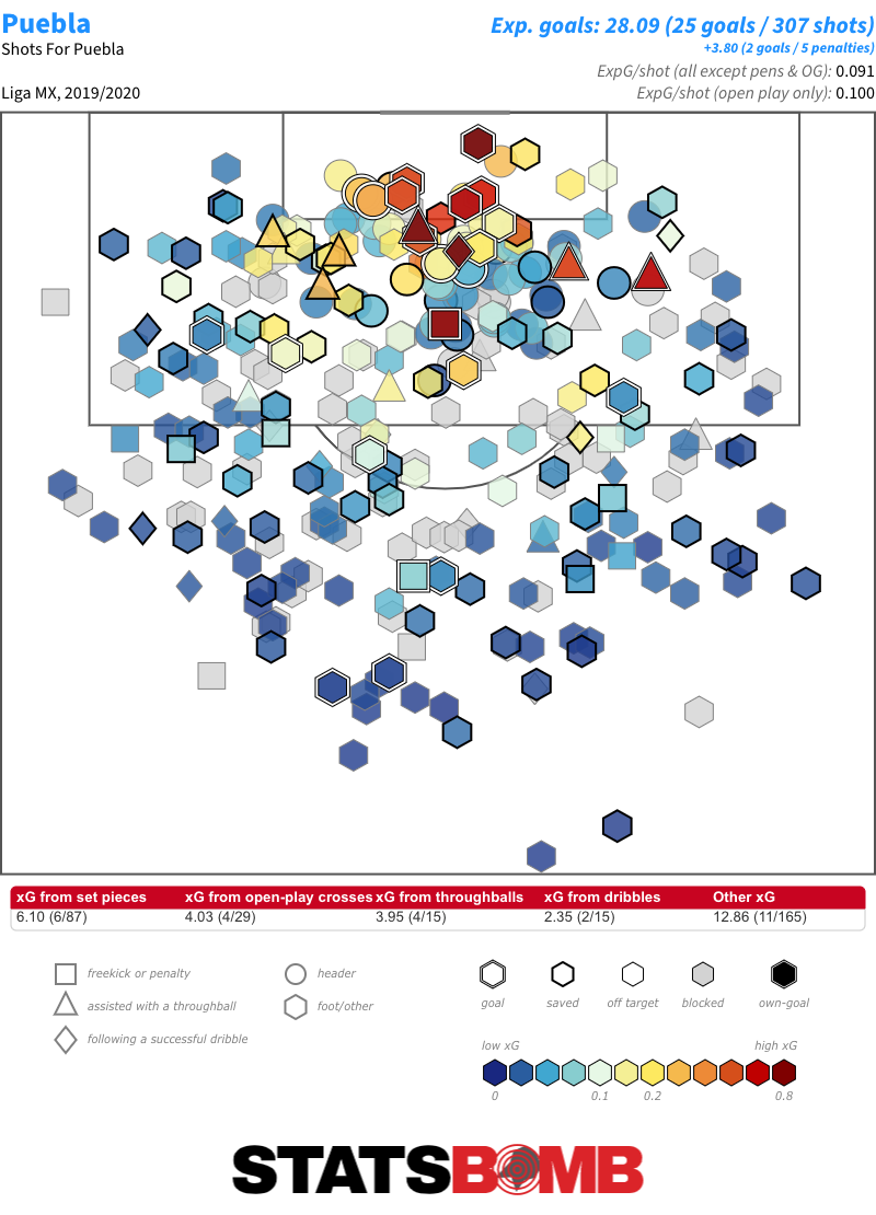 In terms of goals, no team were as lopsided as Necaxa, who scored nearly a quarter of their goals from the right, but only 5.66% from the left. Defensive Styles This graphic shows how each team’s proportion of defensive actions, including StatsBomb’s exclusive pressure data, to opposition passes compares with the league average in each of six vertical zones. The red tones indicate that the team completed an above-average proportion of defensive actions in that zone.
 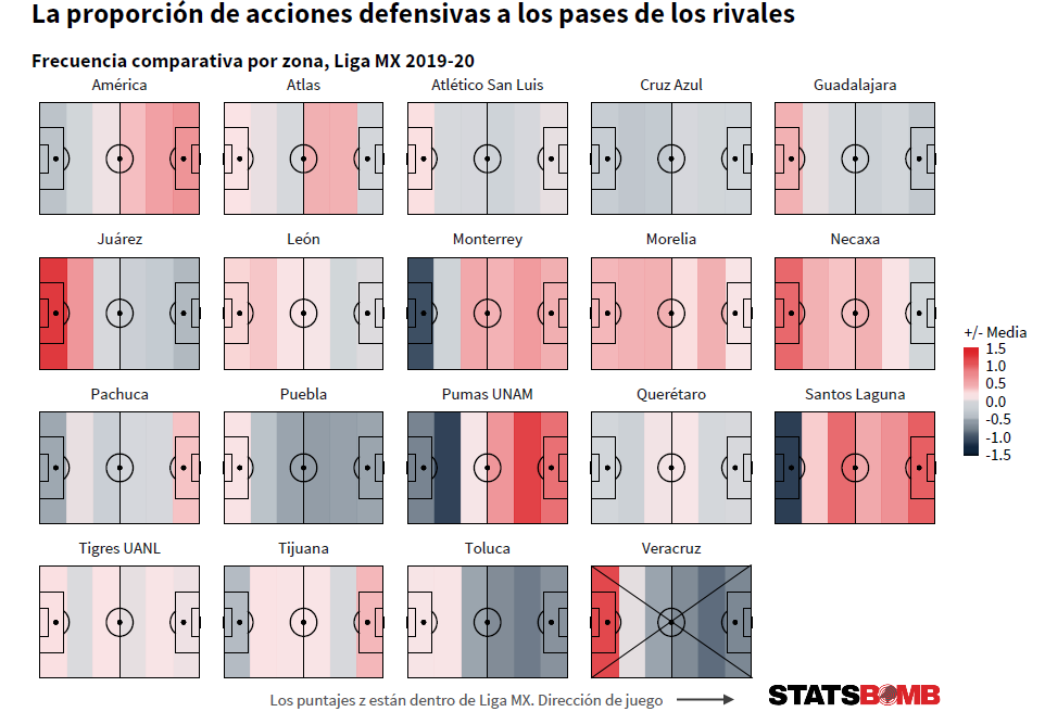 Through this, we can identify groupings of teams with similar defensive styles. If you like proactive teams that defend high up the pitch then Monterrey, Pumas or Santos Laguna might be to your liking. If teams who primarily defend in their own defensive third are your thing then Chivas, Juárez or Toluca might be the ticket. If you’re looking for ones who are pretty much averagely proactive all across the pitch there is always León or Tigres. There is a style for every taste. Talented Young Forwards There were five young forwards, aged 21 or under, who saw at least 900 minutes of action over the course of the truncated 2019-20 season. In order of their combined expected goals and expected goals assisted contribution per 90 minutes, lowest to highest: Diego Abella (Puebla), Germán Berterame (San Luis), José Macías (León/Chivas), Adrián Lozano (Santos Laguna) and Federico Viñas (América). The top two, Lozano and Viñas, have quite different profiles. Lozano is a creator who also posts up solid shot volume; Viñas is an out and out, penalty box centre-forward.
 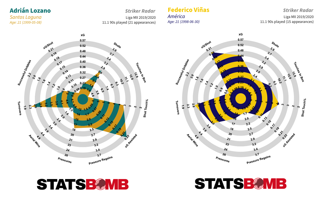 Viñas over-performed his xG tally through the 2019-20 season, converting him into the highest scorer, on a per 90 basis, in the league amongst all players who played at least 900 minutes. But even his xG figure was the second best in the league on that basis.
  Macías is an interesting case. He put up solid numbers at León in the first half of the season (his goal tally was significantly inflated by the five penalties he converted) but then really kicked things up a notch upon returning to his parent club Chivas in January. The question now is if he can maintain that output over a larger sample size.
  One and Two-Footed Players One of the unique features of the StatsBomb data set is that we record the foot with which each pass is played. Over a period of time that allows us to look at which players are the most and least two-footed. During the 2019-20 season, the Pachuca central defender Óscar Murillo was the the most two-footed player in Liga MX. He attempted 49% of his passes with his left foot and 51% with his right.
 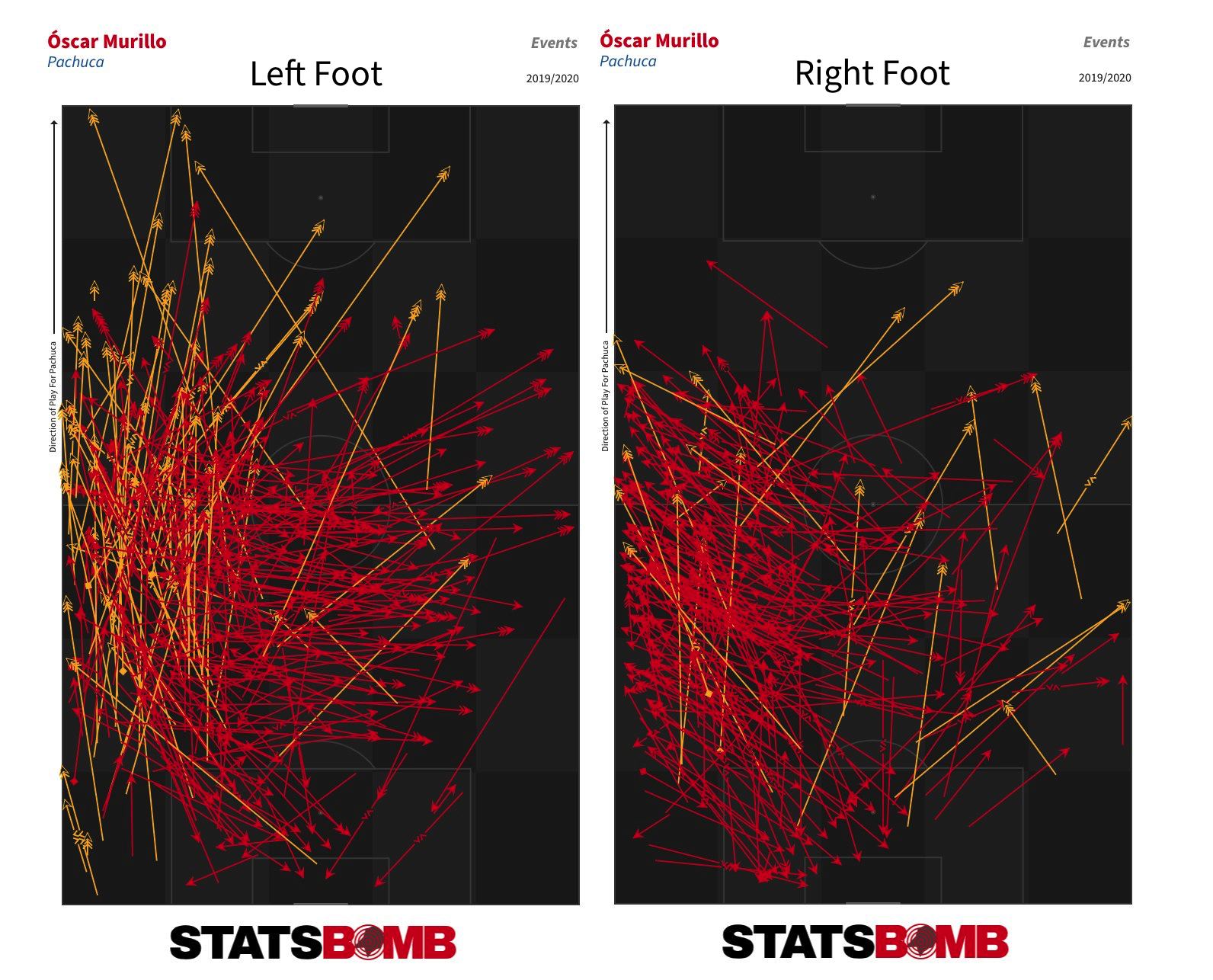 Leonardo Ramos of León and Puebla’s Abella were next up. But who was the least ambidextrous player? Jaime Gómez of Querétaro, who attempted 97% of his passes with his right foot. His teammate Ayron del Valle and León’s Miguel Herrera (now of Pachuca) showed similar skews to their favoured feet. More Stats of Interest If dribblers are your thing, Querétaro were the team to watch last season. Jeison Lucumí and Fabián Castillo were the top two in Liga MX in terms of both attempted and completed dribbles.
 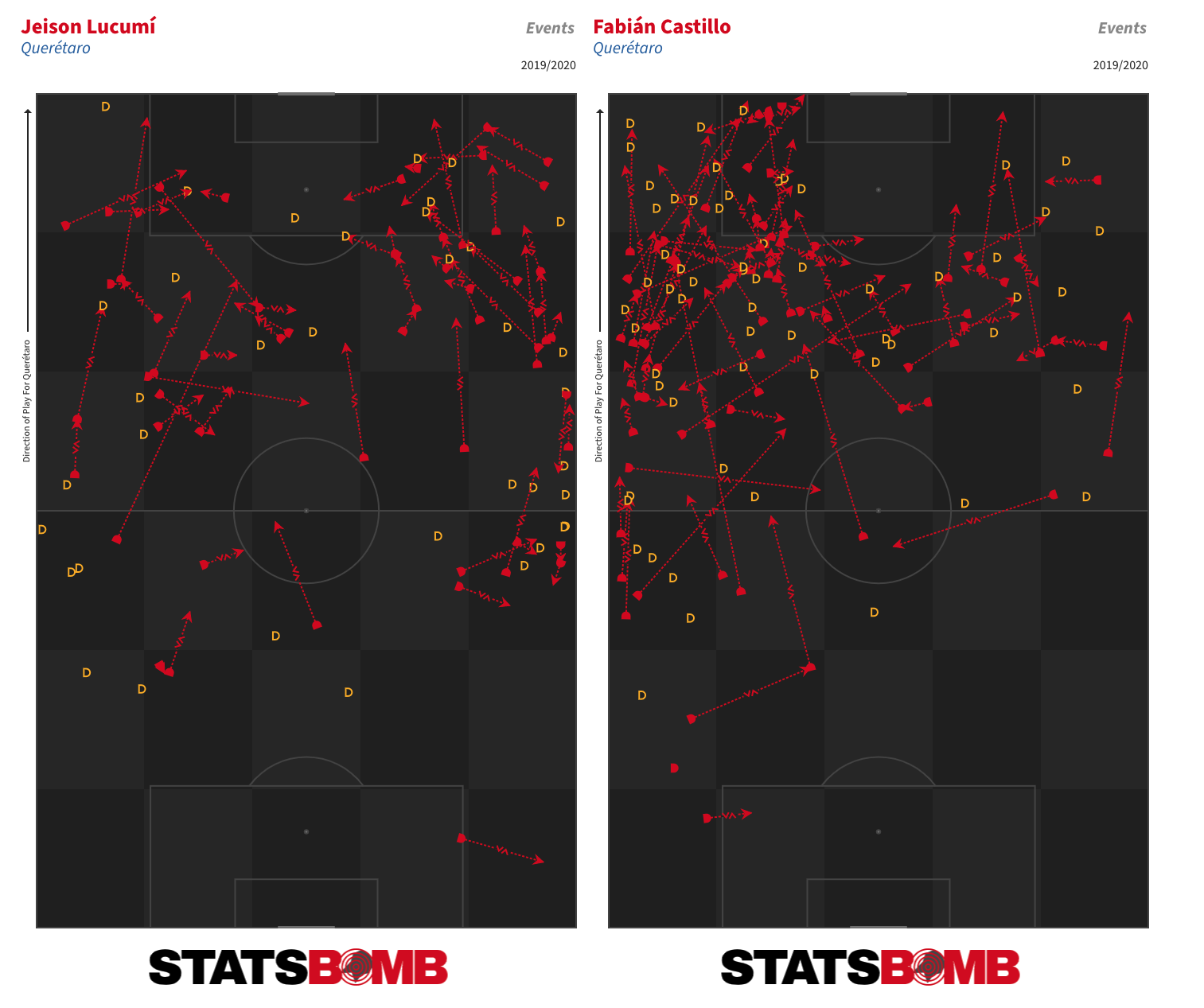 Fernando Gorriarán had the dubious honour of taking the highest number of shots without scoring (46) in Liga MX last season, but the Santos Laguna midfielder was also one of the most defensively active players in the league. Only Luis Quiñones of Tigres and León’s Aquino got through more combined interceptions, pressures and tackles than the Uruguayan on a possession-adjusted basis.
  Rodrigo Noya didn’t react well to being pressed last season. The pass completion rate of the Nexaca central defender dropped from 81% in all situations to 57% when he was put under pressure -- a drop of 26 percentage points than was the highest in the league amongst all outfield players who attempted at least 20 passes per 90.
 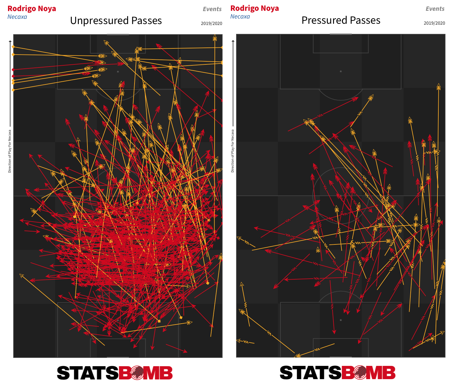 Finally, it was quite clear which teams did the best job of generating chances and goals from set pieces in the 2019-20 season. Cruz Azul, Monterrey, Pumas and Santos Laguna filled the top four places in terms of both set piece xG and set piece goals.
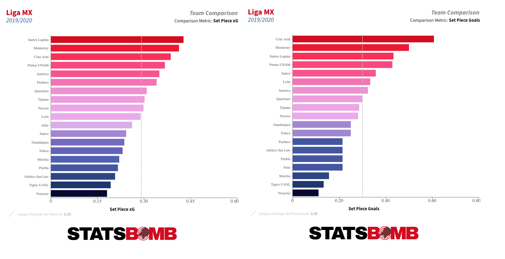
Alongside the release of our Messi dataset we also put a PDF guide to using our data in R. It was intended as a basic introduction to not only our dataset but also the R programming language itself, for those who have yet to use it at any level. Hopefully that gave anyone interested in digging into football data a nice, smooth onboarding to the whole process.
For those who have taken the plunge, this article is going to go through a few more involved things that one could do with the data. This is for those that have already gone through the guide and have been playing about with SBD for a while now. It's important that you have done this first as we will not be walking through absolutely everything and assumes a certain level of familiarity with R. Now that the base terminology of it all has been established it should be easier to explore uncharted territory with a bit less trepidation. So far we have released open data on the women’s and men’s World Cups, the FAWSL, the NWSL, Lionel Messi’s entire La Liga career, the 2003/04 Arsenal Invincibles and 15 years of Champions League finals. You can follow along with this article using any dataset you like but for consistency's sake we will be using the 2019/20 FAWSL season in all examples.
One last disclaimer: this is, of course, all about R. We also have a package for Python that isn’t quite as developed but still handles plenty of the basics for you if that’s your programming language of choice.
A big hurdle to doing anything nuanced with any dataset is one’s underlying understanding of it. There are so many distinct variables and considerations in the SB dataset that even I - having worked with it as my job for two years now - forget about some parts of it every now and then.
To this end it helps to not only have our specs to hand for checking, but also to be aware of the names() and unique() functions. These allow you to get a top-down look at the columns/rows a dataframe contains. So let’s assume you have your data in an R df called ‘events’. We will be using this name for the data in all examples throughout this article. If you were to do names(StatsBombData) that would give you a list of all the columns in your dataset.
Similarly, if you were to do unique(StatsBombData$type.name) you would get a list of every unique row that the ‘type.name’ column contains, i.e all the event types in our data. You can of course do that with any column. It’s good to have these two in your back pocket should you get lost in the forest of data at any point.
xGA, Joining and xG+xGA
xG assisted does not exist in our data initially. However, given that xGA is the xG value of a shot that a key pass/assist created, and that xG values do exist in our data, we can create xGA quite easily via joining. Here’s the code for that, we’ll go through it bit-by-bit afterwards:
library(tidyverse)
library(StatsBombR)
xGA = events %>%
filter(type.name=="Shot") %>% #1
select(shot.key_pass_id, xGA = shot.statsbomb_xg) #2
shot_assists = left_join(events, xGA, by = c("id" = "shot.key_pass_id")) %>% #3
select(team.name, player.name, player.id, type.name, pass.shot_assist, pass.goal_assist, xGA ) %>% #4
filter(pass.shot_assist==TRUE | pass.goal_assist==TRUE) #5
- Filtering the data to just shots, as they are the only events with xG values.
- Select() allows you to choose which columns you want to, well, select, from your data, as not all are always necessary - especially with big datasets. First we are selecting the shot.key_pass_id column, which is a variable attached to shots that is just the ID of the pass that created the shot. You can also rename columns within select() which is what we are doing with xGA = shot.statsbomb_xg. This is so that, when we join it with the passes, it already has the correct name.
- left_join() lets you combine the columns from two different DFs by using two columns within either side of the join as reference keys. So in this example we are taking our initial DF (‘events’) and joining it with the one we just made (‘xGA’). The key is the by = c("id" = "shot.key_pass_id") part, this is saying ‘join these two DFs on instances where the id column in events matches the ‘shot.key_pass_id’ column in xGA’. So now the passes have the xG of the shots they created attached to them under the new column ‘xGA’.
- Again selecting just the relevant columns.
- Filtering our data down to just key passes/assists.
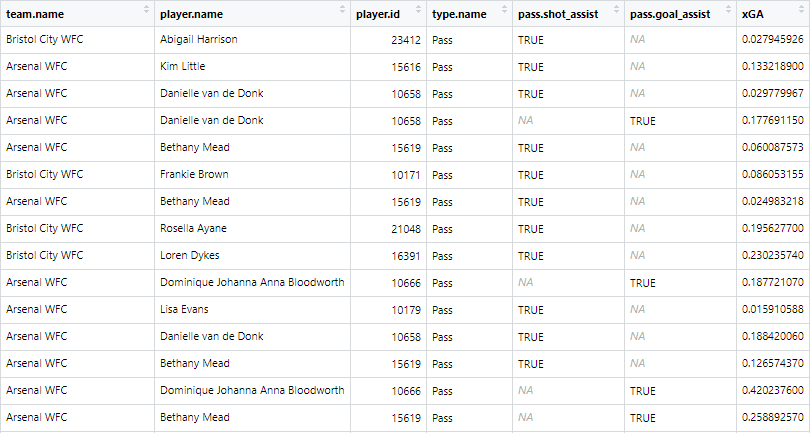
The end result should look like this:
All lovely. But what if you want to make a chart out of it? Say you want to combine it with xG to make a handy xG+xGA per90 chart:
player_xGA = shot_assists %>%
group_by(player.name, player.id, team.name) %>%
summarise(xGA = sum(xGA, na.rm = TRUE)) #1
player_xG = events %>% filter(type.name=="Shot") %>%
filter(shot.type.name!="Penalty" | is.na(shot.type.name)) %>%
group_by(player.name, player.id, team.name) %>%
summarise(xG = sum(shot.statsbomb_xg, na.rm = TRUE)) %>%
left_join(player_xGA) %>% mutate(xG_xGA = sum(xG+xGA, na.rm =TRUE) ) #2
player_minutes = get.minutesplayed(events)
player_minutes = player_minutes %>%
group_by(player.id) %>%
summarise(minutes = sum(MinutesPlayed)) #3
player_xG_xGA = left_join(player_xG, player_minutes) %>%
mutate(nineties = minutes/90, xG_90 = round(xG/nineties, 2),
xGA_90 = round(xGA/nineties,2),
xG_xGA90 = round(xG_xGA/nineties,2) ) #4
chart = player_xG_xGA %>%
ungroup() %>% filter(minutes>=600) %>%
top_n(n = 15, w = xG_xGA90) #5
chart<-chart %>%
select(1, 9:10)%>%
pivot_longer(-player.name, names_to = "variable", values_to = "value") %>%
filter(variable=="xG_90" | variable=="xGA_90") #6
- Grouping by player and summing their total xGA for the season.
- Filtering out penalties and summing each player's xG, then joining with the xGA and adding the two together to get a third combined column.
- Getting minutes played for each player. If you went through the initial R guide you will have done this already.
- Joining the xG/xGA to the minutes, creating the 90s and dividing each stat by the 90s to get xG per 90 etc.
- Here we ungroup as we need the data in ungrouped form for what we're about to do. First we filter to players with a minimum of 600 minutes, just to get rid of notably small samples. Then we use top_n(). This filters your DF to the top *insert number of your choice here* based on a column you specify. So here we're filtering to the top 15 players in terms of xG90+xGA90.
- The pivot_longer() function flattens out the data. It's easier to explain what that means if you see it first:
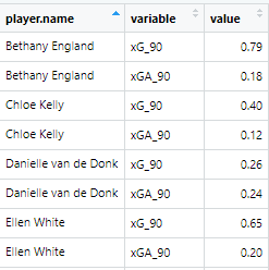
It has used the player.name as a reference point at creates separate rows for every variable that's left over. We then filter down to just the xG90 and xGA90 variables so now each player has a separate variable and value row for those two metrics. Now let's plot it:
ggplot(chart, aes(x =reorder(player.name, value), y = value, fill=fct_rev(variable))) + #1
geom_bar(stat="identity", colour="white")+
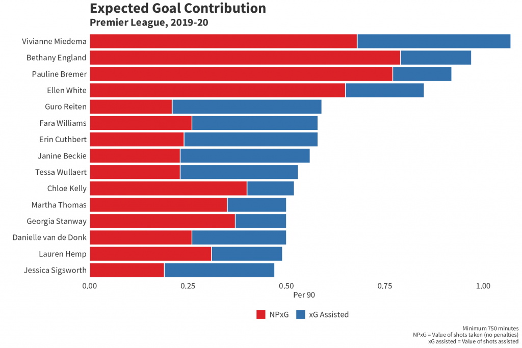
labs(title = "Expected Goal Contribution", subtitle = "Premier League, 2019-20",
x="", y="Per 90", caption ="Minimum 750 minutes\nNPxG = Value of shots taken (no penalties)\nxG assisted = Value of shots assisted")+
theme(axis.text.y = element_text(size=14, color="#333333", family="Source Sans Pro"),
axis.title = element_text(size=14, color="#333333", family="Source Sans Pro"),
axis.text.x = element_text(size=14, color="#333333", family="Source Sans Pro"),
axis.ticks = element_blank(),
panel.background = element_rect(fill = "white", colour = "white"),
plot.background = element_rect(fill = "white", colour ="white"),
panel.grid.major = element_blank(),
panel.grid.minor = element_blank(),
plot.title=element_text(size=24, color="#333333", family="Source Sans Pro" , face="bold"),
plot.subtitle=element_text(size=18, color="#333333", family="Source Sans Pro", face="bold"),
plot.caption=element_text(color="#333333", family="Source Sans Pro", size =10), text=element_text(family="Source Sans Pro"),
legend.title=element_blank(),
legend.text = element_text(size=14, color="#333333", family="Source Sans Pro"),
legend.position = "bottom") + #2
scale_fill_manual(values=c("#3371AC", "#DC2228"), labels = c( "xG Assisted","NPxG")) + #3
scale_y_continuous(expand = c(0, 0), limits= c(0,max(chart$value) + 0.3)) + #4
coord_flip()+ #5
guides(fill = guide_legend(reverse = TRUE)) #6
- Two things are going on here that are different from your average bar chart. First is reorder(), which allows you reorder a variable along either axis based on a second variable. In this instance we are putting the player names on the x axis and reordering them by value - i.e the xG and xGA combined - meaning they are now in descending order from most to least combined xG+xGA. Second is that we've put the 'variable' on the bar fill. This allows us to put two separate metrics onto one bar chart and have them stack, as you will see below, by having them be separate fill colours.
- Everything within labs() and theme() is fairly self explanatory and is just what we have used internally. You can get rid of all this if you like and change it to suit your own design tastes.
- Here we are providing specific colour hex codes to the values (so xG = red and xGA = blue) and then labelling them so they are named correctly on the chart's legend.
- Expand() allows you to expand the boundaries of the x or y axis, but if you set the values to (0,0) it also removes all space between the axis and the inner chart itself (if you're having a hard time envisioning that, try removing expand() and see what it looks like). Then we are setting the limits of the y axis so the longest bar on the chart isn't too close to the edge of the chart. 'max(chart$value) + 0.3' is saying 'take the max value and add 0.3 to make that the upper limit of the y axis'.
- Flipping the x axis and y axis so we have a nice horizontal bar chart rather than a vertical one.
- Reversing the legend so that the order of it matches up with the order of xG and xGA on the chart itself.
All in that should look like this:
Heatmaps
Heatmaps are one of the everpresents in football data. They are fairly easy to make in R once you get your head round how to do so, but can be unintuitive without having it explained to you first. For this example we're going to do a defensive heatmap, looking at how often teams make a % of their overall defensive actions in certain zones, then comparing that % vs league average:
library(tidyverse)
heatmap = events %>%
mutate(location.x = ifelse(location.x>120, 120, location.x),
location.y = ifelse(location.y>80, 80, location.y),
location.x = ifelse(location.x<0, 0, location.x),
location.y = ifelse(location.y<0, 0, location.y)) #1
heatmap$xbin <- cut(heatmap$location.x, breaks = seq(from=0, to=120, by = 20),include.lowest=TRUE )
heatmap$ybin <- cut(heatmap$location.y, breaks = seq(from=0, to=80, by = 20),include.lowest=TRUE) #2
heatmap = heatmap%>%
filter(type.name=="Pressure" | duel.type.name=="Tackle" | type.name=="Foul Committed" | type.name=="Interception" |
type.name=="Block" ) %>%
group_by(team.name) %>%
mutate(total_DA = n()) %>%
group_by(team.name, xbin, ybin) %>%
summarise(total_DA = max(total_DA),
bin_DA = n(),
bin_pct = bin_DA/total_DA,
location.x = median(location.x),
location.y = median(location.y)) %>%
group_by(xbin, ybin) %>%
mutate(league_ave = mean(bin_pct)) %>%
group_by(team.name, xbin, ybin) %>%
mutate(diff_vs_ave = bin_pct - league_ave) #3
- Some of the coordinates in our data sit outside the bounds of the pitch (you can see the layout of our pitch coordinates in our event spec, but it's 0-120 along the x axis and 0-80 along the y axis). This will cause issue with a heatmap and give you dodgy looking zones outside the pitch. So what we're doing here is using ifelse() to say 'if a location.x/y coordinate is outside the bounds that we want, then replace it with one that's within the boundaries. If it is not outside the bounds just leave it as is'.
- cut() literally cuts up the data how you ask it to. Here, we're cutting along the x axis (from 0-120, again the length of our pitch according to our coordinates in the spec) and the y axis (0-80), and we're cutting them 'by' the value we feed it, in this case 20. So we're splitting it up into buckets of 20. This creates 6 buckets/zones along the x axis (120/20 = 6) and 4 along the y axis (80/20 = 4). This creates the buckets we need to plot our zones.
- This is using those buckets to create the zones. Let's break it down bit-by-bit: - Filtering to only defensive events - Grouping by team and getting how many defensive events they made in total ( n() just counts every row that you ask it to, so here we're counting every row for every team - i.e counting every defensive event for each team) - Then we group again by team and the xbin/ybin to count how many defensive events a team has in a given bin/zone - that's what 'bin_DA = n()' is doing. 'total_DA = max(total_DA),' is just grabbing the team totals we made earlier. 'bin_pct = bin_DA/total_DA,' is dividing the two to see what percentage of a team's overall defensive events were made in a given zone. The 'location.x = median(location.x/y)' is doing what it says on the tin and getting the median coordinate for each zone. This is used later in the plotting. - Then we ungroup and mutate to find the league average for each bin, followed by grouping by team/bin again subtracting the league average in each bin from each team's % in those bins to get the difference.
Now onto the plotting. For this please install the package 'grid' if you do not have it, and load it in. You could use a package like 'ggsoccer' or 'SBPitch' for drawing the pitch, but for these purposes it's helpful to try and show you how to create your own pitch, should you want to:
library(grid)
defensiveactivitycolors <- c("#dc2429", "#dc2329", "#df272d", "#df3238", "#e14348", "#e44d51", "#e35256", "#e76266", "#e9777b", "#ec8589", "#ec898d", "#ef9195", "#ef9ea1", "#f0a6a9", "#f2abae", "#f4b9bc", "#f8d1d2", "#f9e0e2", "#f7e1e3", "#f5e2e4", "#d4d5d8", "#d1d3d8", "#cdd2d6", "#c8cdd3", "#c0c7cd", "#b9c0c8", "#b5bcc3", "#909ba5", "#8f9aa5", "#818c98", "#798590", "#697785", "#526173", "#435367", "#3a4b60", "#2e4257", "#1d3048", "#11263e", "#11273e", "#0d233a", "#020c16") #1
ggplot(data= heatmap, aes(x = location.x, y = location.y, fill = diff_vs_ave, group =diff_vs_ave)) +
geom_bin2d(binwidth = c(20, 20), position = "identity", alpha = 0.9) + #2
annotate("rect",xmin = 0, xmax = 120, ymin = 0, ymax = 80, fill = NA, colour = "black", size = 0.6) +
annotate("rect",xmin = 0, xmax = 60, ymin = 0, ymax = 80, fill = NA, colour = "black", size = 0.6) +
annotate("rect",xmin = 18, xmax = 0, ymin = 18, ymax = 62, fill = NA, colour = "white", size = 0.6) +
annotate("rect",xmin = 102, xmax = 120, ymin = 18, ymax = 62, fill = NA, colour = "white", size = 0.6) +
annotate("rect",xmin = 0, xmax = 6, ymin = 30, ymax = 50, fill = NA, colour = "white", size = 0.6) +
annotate("rect",xmin = 120, xmax = 114, ymin = 30, ymax = 50, fill = NA, colour = "white", size = 0.6) +
annotate("rect",xmin = 120, xmax = 120.5, ymin =36, ymax = 44, fill = NA, colour = "black", size = 0.6) +
annotate("rect",xmin = 0, xmax = -0.5, ymin =36, ymax = 44, fill = NA, colour = "black", size = 0.6) +
annotate("segment", x = 60, xend = 60, y = -0.5, yend = 80.5, colour = "white", size = 0.6)+
annotate("segment", x = 0, xend = 0, y = 0, yend = 80, colour = "black", size = 0.6)+
annotate("segment", x = 120, xend = 120, y = 0, yend = 80, colour = "black", size = 0.6)+
theme(rect = element_blank(), line = element_blank()) +
annotate("point", x = 12 , y = 40, colour = "white", size = 1.05) + # add penalty spot right
annotate("point", x = 108 , y = 40, colour = "white", size = 1.05) +
annotate("path", colour = "white", size = 0.6, x=60+10*cos(seq(0,2*pi,length.out=2000)),
y=40+10*sin(seq(0,2*pi,length.out=2000)))+ # add centre spot
annotate("point", x = 60 , y = 40, colour = "white", size = 1.05) +
annotate("path", x=12+10*cos(seq(-0.3*pi,0.3*pi,length.out=30)), size = 0.6,
y=40+10*sin(seq(-0.3*pi,0.3*pi,length.out=30)), col="white") +
annotate("path", x=108-10*cos(seq(-0.3*pi,0.3*pi,length.out=30)), size = 0.6,
y=40-10*sin(seq(-0.3*pi,0.3*pi,length.out=30)), col="white") + #3
theme(axis.text.x=element_blank(),
axis.title.x = element_blank(),
axis.title.y = element_blank(),
plot.caption=element_text(size=13,family="Source Sans Pro", hjust=0.5, vjust=0.5),
plot.subtitle = element_text(size = 18, family="Source Sans Pro", hjust = 0.5),
axis.text.y=element_blank(),
legend.title = element_blank(),
legend.text=element_text(size=22,family="Source Sans Pro"),
legend.key.size = unit(1.5, "cm"),
plot.title = element_text(margin = margin(r = 10, b = 10), face="bold",size = 32.5, family="Source Sans Pro", colour = "black", hjust = 0.5),
legend.direction = "vertical",
axis.ticks=element_blank(),
plot.background = element_rect(fill = "white"),strip.text.x = element_text(size=13,family="Source Sans Pro")) + #4
scale_y_reverse() + #5
scale_fill_gradientn(colours = defensiveactivitycolors, trans = "reverse", labels = scales::percent_format(accuracy = 1), limits = c(0.02, -0.02)) + #6
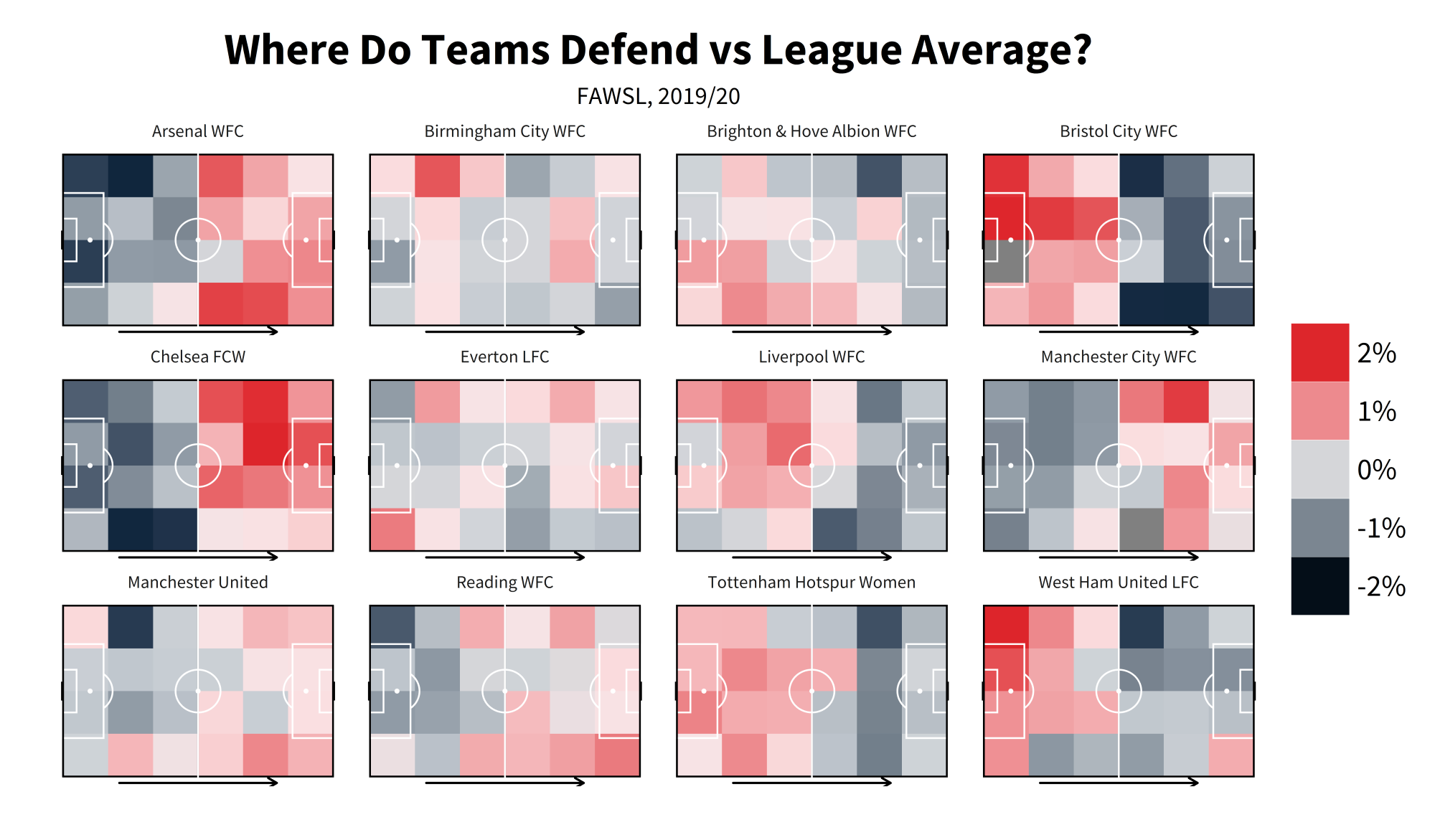
labs(title = "Where Do Teams Defend vs League Average?", subtitle = "FAWSL, 2019/20") + #7
coord_fixed(ratio = 95/100) + #8
annotation_custom(grob = linesGrob(arrow=arrow(type="open", ends="last", length=unit(2.55,"mm")), gp=gpar(col="black", fill=NA, lwd=2.2)), xmin=25, xmax = 95, ymin = -83, ymax = -83) + #9
facet_wrap(~team.name)+ #10
guides(fill = guide_legend(reverse = TRUE)) #11
- These are the colours we'll be using for our heatmap later on.
- 'geom_bin2d' is what will create the heatmap itself. We've set the binwidths to 20 as that's what we cut the pitch up into earlier along the x and y axis. Feeding 'div_vs_ave' to 'fill' and 'group' in the ggplot() will allow us to colour the heatmaps by that variable.
- Everything up to here is what is drawing the pitch. There's a lot going on here and, rather than have it explained to you, just delete a line from it and see what disappears from the plot. Then you'll see which line is drawing the six-yard-box, which is drawing the goal etc.
- Again more themeing. You can change this to be whatever you like to fit your aesthetic preferences.
- Reversing the y axis so the pitch is the correct way round along that axis (0 is left in SBD coordinates, but starts out as right in ggplot).
- Here we're setting the parameters for the fill colouring of heatmaps. First we're feeding the 'defensiveactivitycolors' we set earlier into the 'colours' parameter, 'trans = "reverse"' is there to reverse the output so red = high. 'labels = scales::percent_format(accuracy = 1)' formats the text on the legend as a percentage rather than a raw number and 'limits = c(0.03, -0.03)' sets the limits of the chart to 3%/-3% (reversed because of the previous trans = reverse).
- Setting the title and subtitle of the chart.
- 'coord_fixed()' allows us to set the aspect ratio of the chart to our liking. Means the chart doesn't come out looking all stretched along one of the axes.
- This is what the grid package is used for. It's drawing the arrow across the pitches to indicate direction of play. There's multiple ways you could accomplish though, up to you how you do it.
- 'facet_wrap()' creates separate 'facets' for your chart according to the variable you give it. Without it, we'd just be plotting every team's numbers all at once on chart. With it, we get every team on their own individual pitch.
- Our previous trans = reverse also reverses the legend, so to get it back with the positive numbers pointing upwards we can re-reverse it.
Shot Maps
Another of the quintessential football visualisations, shot maps come in many shapes and sizes with an inconsistent overlap in design language between them. This version will attempt to give you the basics, let you get to grip with how to put one of these together so that if you want to elaborate or make any of your own changes you can explore outwards from it. Be forewarned though - the options for what makes a good, readable shot map are surprisingly small when you get into visualising it!
shots = events %>%
filter(type.name=="Shot" & (shot.type.name!="Penalty" | is.na(shot.type.name)) & player.name=="Bethany England") #1
shotmapxgcolors <- c("#192780", "#2a5d9f", "#40a7d0", "#87cdcf", "#e7f8e6", "#f4ef95", "#FDE960", "#FCDC5F", "#F5B94D", "#F0983E", "#ED8A37", "#E66424", "#D54F1B", "#DC2608", "#BF0000", "#7F0000", "#5F0000") #2
ggplot() +
annotate("rect",xmin = 0, xmax = 120, ymin = 0, ymax = 80, fill = NA, colour = "black", size = 0.6) +
annotate("rect",xmin = 0, xmax = 60, ymin = 0, ymax = 80, fill = NA, colour = "black", size = 0.6) +
annotate("rect",xmin = 18, xmax = 0, ymin = 18, ymax = 62, fill = NA, colour = "black", size = 0.6) +
annotate("rect",xmin = 102, xmax = 120, ymin = 18, ymax = 62, fill = NA, colour = "black", size = 0.6) +
annotate("rect",xmin = 0, xmax = 6, ymin = 30, ymax = 50, fill = NA, colour = "black", size = 0.6) +
annotate("rect",xmin = 120, xmax = 114, ymin = 30, ymax = 50, fill = NA, colour = "black", size = 0.6) +
annotate("rect",xmin = 120, xmax = 120.5, ymin =36, ymax = 44, fill = NA, colour = "black", size = 0.6) +
annotate("rect",xmin = 0, xmax = -0.5, ymin =36, ymax = 44, fill = NA, colour = "black", size = 0.6) +
annotate("segment", x = 60, xend = 60, y = -0.5, yend = 80.5, colour = "black", size = 0.6)+
annotate("segment", x = 0, xend = 0, y = 0, yend = 80, colour = "black", size = 0.6)+
annotate("segment", x = 120, xend = 120, y = 0, yend = 80, colour = "black", size = 0.6)+
theme(rect = element_blank(), line = element_blank()) + # add penalty spot right
annotate("point", x = 108 , y = 40, colour = "black", size = 1.05) +
annotate("path", colour = "black", size = 0.6, x=60+10*cos(seq(0,2*pi,length.out=2000)),
y=40+10*sin(seq(0,2*pi,length.out=2000)))+ # add centre spot
annotate("point", x = 60 , y = 40, colour = "black", size = 1.05) +
annotate("path", x=12+10*cos(seq(-0.3*pi,0.3*pi,length.out=30)), size = 0.6,
y=40+10*sin(seq(-0.3*pi,0.3*pi,length.out=30)), col="black") +
annotate("path", x=107.84-10*cos(seq(-0.3*pi,0.3*pi,length.out=30)), size = 0.6,
y=40-10*sin(seq(-0.3*pi,0.3*pi,length.out=30)), col="black") +
geom_point(data = shots, aes(x = location.x, y = location.y, fill = shot.statsbomb_xg, shape = shot.body_part.name), size = 6, alpha = 0.8) + #3
theme(axis.text.x=element_blank(),
axis.title.x = element_blank(),
axis.title.y = element_blank(),
plot.caption=element_text(size=13,family="Source Sans Pro", hjust=0.5, vjust=0.5),
plot.subtitle = element_text(size = 18, family="Source Sans Pro", hjust = 0.5),
axis.text.y=element_blank(), legend.position = "top",
legend.title=element_text(size=22,family="Source Sans Pro"),
legend.text=element_text(size=20,family="Source Sans Pro"),
legend.margin = margin(c(20, 10, -85, 50)),
legend.key.size = unit(1.5, "cm"),
plot.title = element_text(margin = margin(r = 10, b = 10), face="bold",size = 32.5, family="Source Sans Pro", colour = "black", hjust = 0.5),
legend.direction = "horizontal",
axis.ticks=element_blank(), aspect.ratio = c(65/100),
plot.background = element_rect(fill = "white"), strip.text.x = element_text(size=13,family="Source Sans Pro")) +
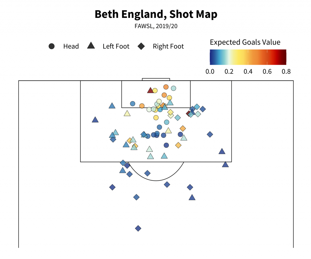
labs(title = "Beth England, Shot Map", subtitle = "FAWSL, 2019/20") + #4
scale_fill_gradientn(colours = shotmapxgcolors, limit = c(0,0.8), oob=scales::squish, name = "Expected Goals Value") + #5
scale_shape_manual(values = c("Head" = 21, "Right Foot" = 23, "Left Foot" = 24), name ="") + #6
guides(fill = guide_colourbar(title.position = "top"), shape = guide_legend(override.aes = list(size = 7, fill = "black"))) + #7 coord_flip(xlim = c(85, 125)) #8
- Simple filtering, leaving out penalties. Choose any player you like of course.
- Much like the defensive activity colours earlier, these will set the colours for our xG values.
- Here's where the actual plotting of shots comes in, via geom_point. We're using the the xG values as the fill and the body part for the shape of the points. This could reasonably be anything though. You could even add in colour parameters which would change the colour of the outline of the shape.
- Again titling. This can be done dynamically so that it changes according to the player/season etc but we will leave that for now. Feel free to explore for youself though.
- Same as last time but worth pointing out that 'name' allows you to change the title of a legend from within the gradient setting.
- Setting the shapes for each body part name. The shape numbers correspond to ggplot's pre-set shapes. The shapes numbered 21 and up are the ones which have inner colouring (controlled by fill) and outline colouring (controlled by colour) so that's why those have been chosen here. oob=scales::squish takes any values that are outside the bounds of our limits and squishes them within them.
- guides() allows you to alter the legends for shape, fill and so on. Here we are changing the the title position for the fill so that it is positioned above the legend, as well as changing the size and colour of the shape symbols on that legend.
- coord_flip() does what it says on the tin - switches the x and y axes. xlim allows us to set boundaries for the x axis so that we can show only a certain part of the pitch, giving us:
That's all for now. Hopefully this wasn't all too confusing and you picked up some bits and bobs you can take away to play with yourselves. Don't worry if some of this is overwhelming or you have to do copious amounts of googling to overcome odd specific errors and whatnot. That's just part and parcel with coding (seriously, get used to googling for errors, everyone has to).
Much love. Be well and have great days.
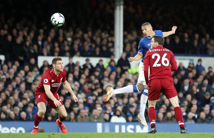
It's reasonable to think that headers have been somewhat overlooked by the analytics community as attention progressed from shooting towards passing, pressing and dribbling. Despite this, they remain an important component of the game with strong variations between competitions across the world. In this article we're looking at a variety of recent league seasons, covering the wide range of competitions that StatsBomb collects.
Analysis
Presented below is the average number of headers per game for each competition split by season. I grouped the competitions to aid comparison and kept the scale constant for each visualisation. Competitions are ordered by their average across the seasons shown.
England & Scotland
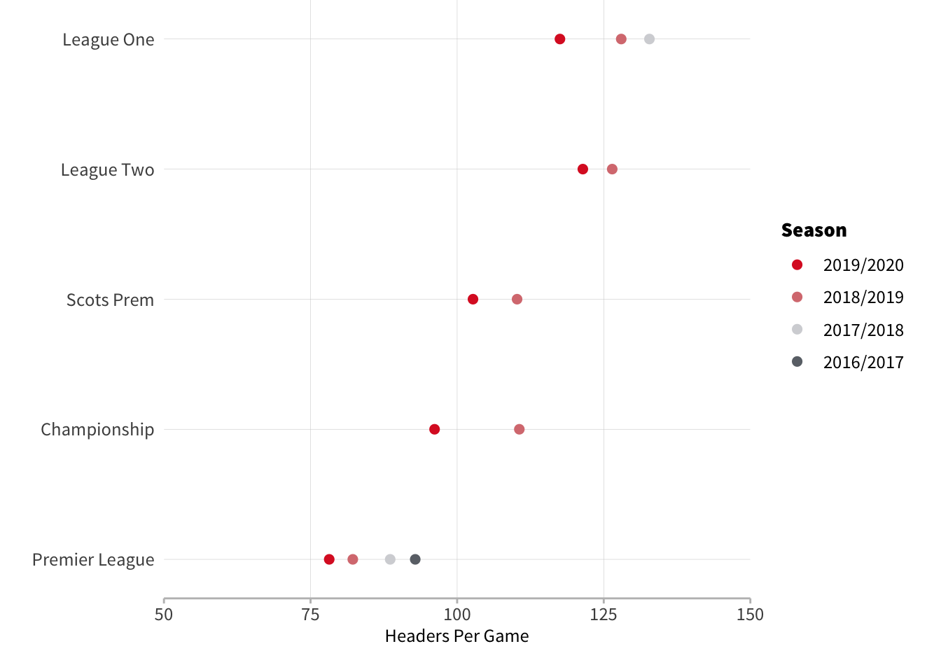
No surprises with the British competitions and we can see a consistent increase in the number of headers per game as we go down the tiers.
There’s actually not much difference once you get down to League 1 and League 2, and in 2018/19 both leagues saw roughly 40 extra headers each game than the Premier League. Indeed, League 2 is responsible for the highest number of headers recorded in a match per our dataset - Macclesfield v Northampton this season had 235 headers equating to roughly one every 23 seconds. If you’re struggling to believe that a professional football match had this many headers then watching the first 30 seconds of the match should clear up any doubts:
The lowest number of headers is the 10 from PSG v Nice last season. Typically the variation between games isn’t as extreme as those edge cases. The standard deviation on a game by game basis ranges from 15 in Colombia’s first tier to 30 in the Scottish Premiership.
The Big 5
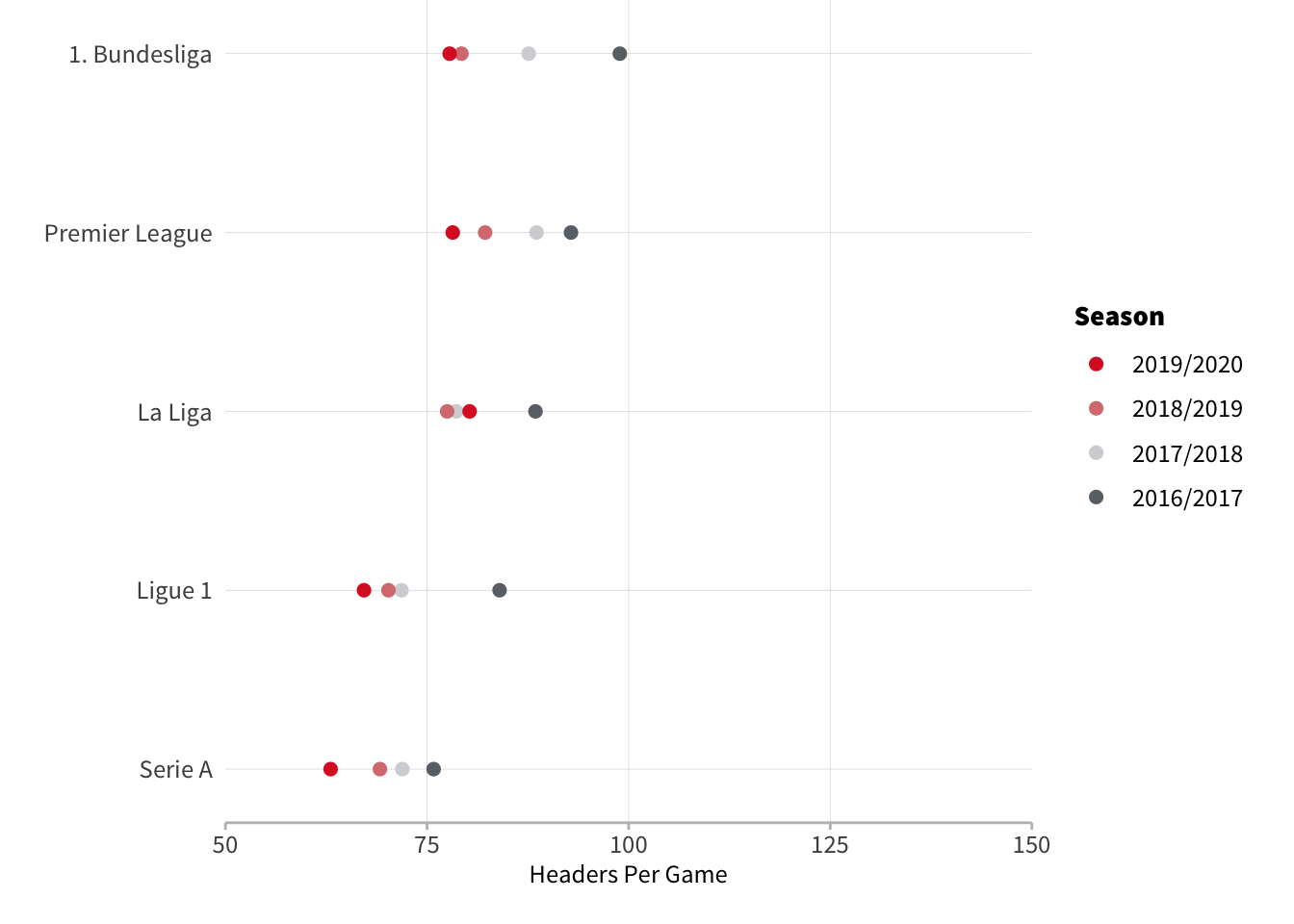
Across the Big 5 we can see the Premier League, Bundesliga and La Liga showing very similar heading tendencies whilst Ligue 1 and Serie A appear to occupy their own group with slightly less heading than the other three.
The Rest of Europe

Most European leagues are hovering around 75 headers per game which aligns more with the Big 5 than what we see in the UK’s lower tiers but there are pockets of stylistic difference, namely in the Austrian Bundesliga and Czech Liga.
Second Tiers
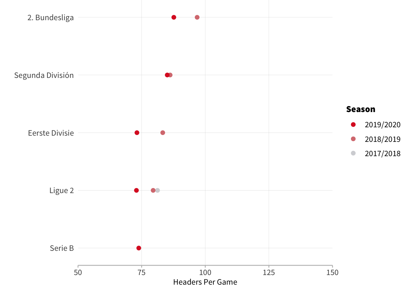
Looking at second tiers we see both Germany and Spain average more headers in their second tier than their top league which mirrors what we see in England. Elsewhere, France, Italy and the Netherlands however have similar averages in their second tier as they do in their top league implying style of play is more consistent across levels in those countries.
Americas and Australia
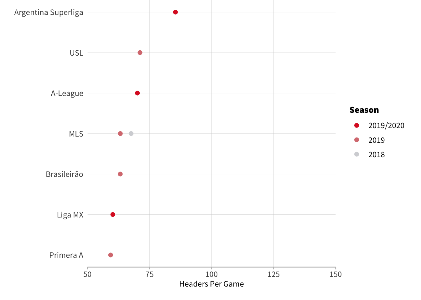
These leagues represent the least aerially active competitions in the men's game - Colombia and Mexico in particular see very few headers. Interestingly, Argentina sets itself part from the other two South American countries with roughly 20 more headers per game.
Women’s Football
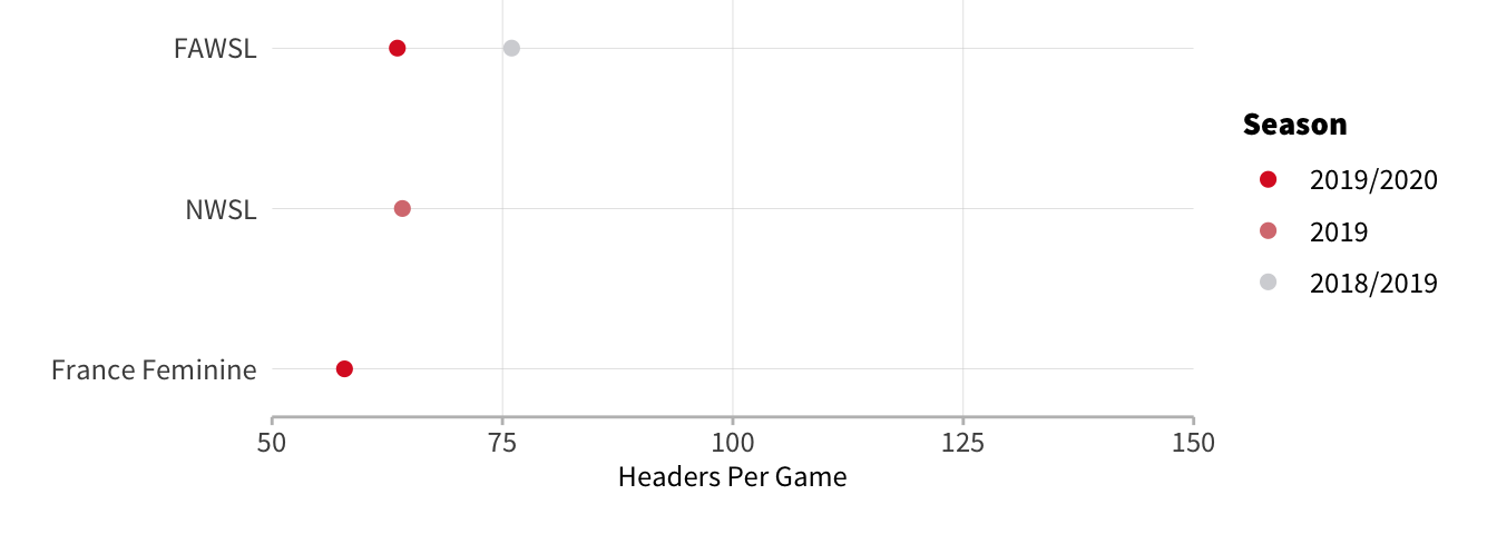
All three competitions have low header numbers, similar to what we saw in the Americas. France actually has the lowest number headers per game in the dataset ahead of the mens' leagues in Colombia and Mexico.
Spatial Trends
Let's see if there are any locational differences between the leagues covered here:
Men’s Competitions
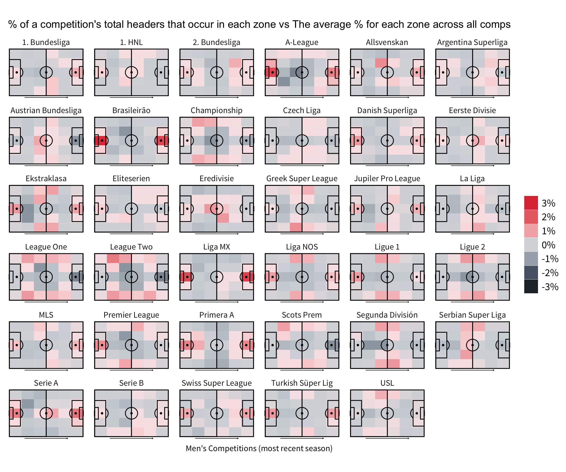
First thing to note is that there’s really not much difference between leagues in terms where their headers take place. At most you’re looking at a three percentage point difference for a zone. That being said, there are a few noticeable clusters.
Firstly, you’ve got the leagues that have a higher proportion of headers inside the box such as Brazil and Mexico. Both these leagues had very low overall header numbers and it seems that heading in those leagues mostly comes from crosses into the box. The UK leagues all show similar patterns with more headers coming in the channels where you would expect the fullbacks to be. If you watch UK lower league football you’ll notice that there’s a lot more long balls into the channel and this seems to support that pattern.
The final cluster has more headers around the half-way line than normal - France, Netherlands, Austria. I’m not totally sure why this might occur, maybe those leagues are willing to clear the ball back the half way line more or aim long goal kicks there more frequently.
By Region
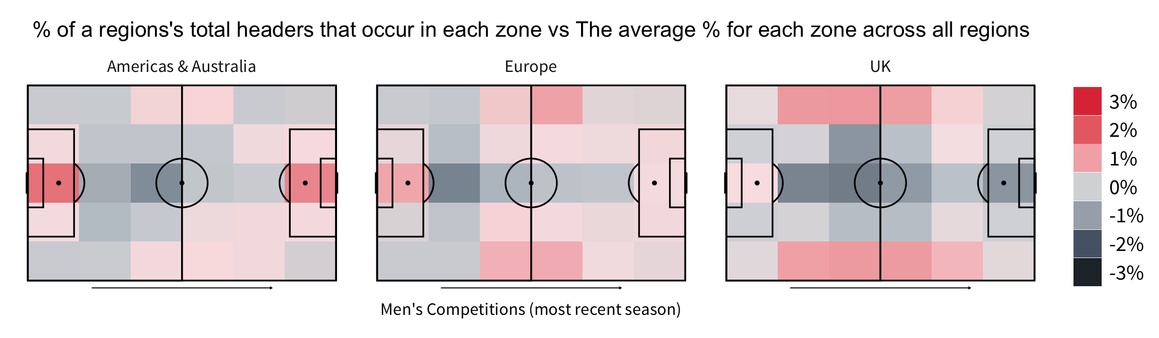
Grouping the competitions by region further highlights these differences - there really are no leagues quite like the UK!
Women’s Competitions
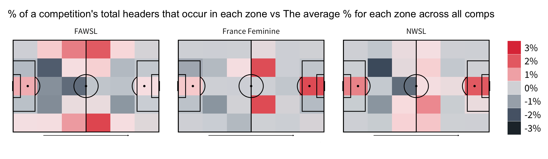 Looking at the women’s leagues reveals three different patterns. It appears heading is slightly different across each of these leagues.
The FAWSL seems to be similar to what we see in the UK’s male leagues with more headers in the channels but they are concentrated around the half way line here. France has a pattern that we haven’t seen before with hot zones in the opposition half. It is possible that the team in possession winning more attacking headers in this league.
The locations of these zones suggest they win these attacking headers from goal kicks and crosses more than usual. In America, we can see a similar pattern to Brazil and Mexico with more headers in each box.
Wider Trends
Finally, you may have noticed in the first section that for leagues in which we have more than one season, headers per game seems to be going down and this is correct. Within the leagues and seasons covered here are 30 instances of a league having less headers per game the following season and only 3 instances of a league having more headers.
Only Belgium, Austria and Spanish La Liga saw an increase in the number of headers this season compared to last. This is an overwhelming trend that can surely only be explained as an evolution of tactical preference and would bear further analysis. This could be through less crossing or in build up play - we already know crossing can be an inefficient form of attack if overprioritised so perhaps teams are catching on to this. It will be interesting to monitor this trend over the next few years.
In this week’s La Liga roundup we look at Valencia’s dismissal of Albert Celades and Arthur’s departure from Barcelona. Results Finally Catch Up With Celades Here’s an idea for wannabe football club owners: don’t impose unworkable conditions on a coach who leads your team to consecutive top-four finishes and its first silverware in over a decade. If you really must persist, definitely don’t replace them with a coach of questionable merit and experience. If you do, this might happen: 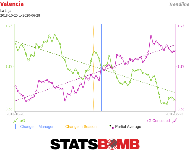 Until recently, Valencia’s results since Albert Celades replaced Marcelino back in mid-September were pretty good. When the league was paused in March, they were seventh in the table, just four points shy of the top four. But the underlying numbers always told a different story, one that results since the restart more accurately reflect. Three defeats in four left Valencia eight points off the top four and Celades without a job. We don’t even really need to dig as deep as expected goals to understand how bad Valencia were under Celades. They took just 8.28 shots per match, the second-lowest tally in the league, and matched that to a league-worst 15.52 conceded. It doesn’t take a genius to work out that giving up seven more shots than you take each week isn’t exactly a formula for sustained success. Back in the days when Total Shots Ratio ruled the analytics roost, we’d probably have considered any team with a shot share of 40% or less to be pretty bad; Valencia under Celades had just a 35% share. If we bring xG into the equation, their average shot quality was better than the quality of those they conceded, but the difference was nowhere near big enough to balance such a large disparity in shot volume. They combined the fourth-lowest xG per match (0.89) with the second-highest xG conceded (1.35) for the third-worst xG difference (-0.46) in the division. Those are the numbers of relegation candidates rather than European aspirants. Results hid those issues. Valencia consistently over-performed their underlying numbers. Even with their slowdown post-restart, they were still running almost nine goals ahead of expectation when Celades was relieved of his duties.
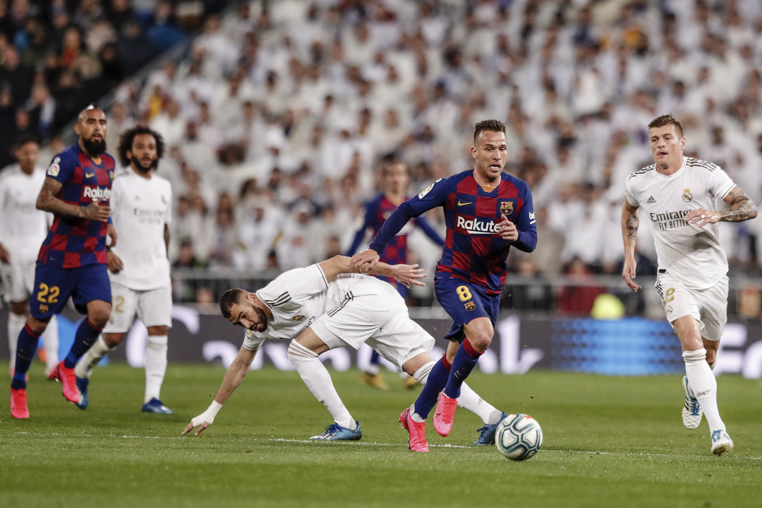
 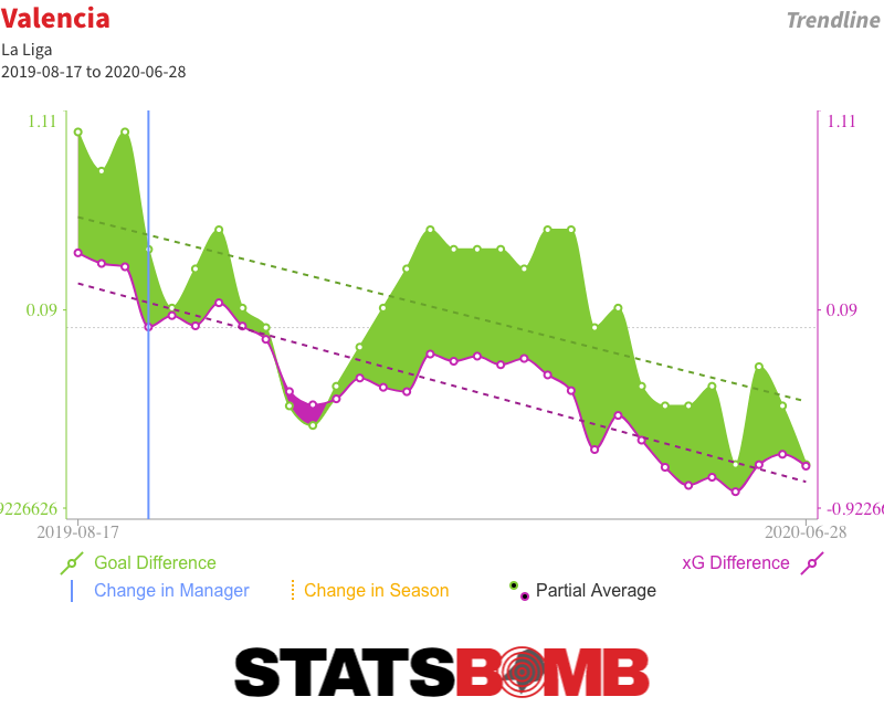 As is almost always the case, there have been attempts to create a narrative arc, to say that things were okay until injuries took hold or to identify a tipping point when control of the dressing room was lost. But the truth is that Valencia were never very good under Celades. It just took a little while for results to reflect that reality. Arthur Leaves, Barcelona Get Older Still Consecutive draws against Celta Vigo and Atlético Madrid have probably ended Barcelona’s challenge for La Liga. Even if they win all five of their remaining matches, Real Madrid can afford to drop four points in their remaining six and still claim the title thanks to their superior head-to-head record. Off the pitch, Barcelona have this week confirmed what essentially amounts to a swap deal with Juventus that will see the Italian club pay an initial €72 million for Arthur at the same time as Barcelona put down €60 million for Miralem Pjanic. It is not a move that makes much sporting sense. The two players have performed different roles this season, which complicates a direct comparison. But even if we accept that stylistic differences aside they are probably about par in terms of present ability, it remains difficult to form a cogent argument for swapping a soon-to-be 24-year-old for a 30-year-old. Particularly when Barcelona already have a large contingent of post-peak players gobbling up minutes.
 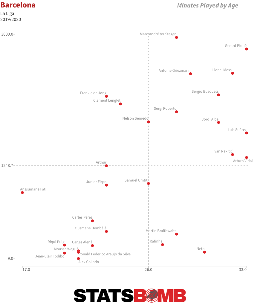 The truth is that this deal isn’t about what happens on the pitch; it’s about moving around figures on a spreadsheet to balance budgets. Both teams had deficits to make up and constructed a mutual means of doing so. Alternative scenarios that revolve around Barcelona selling Arthur but reinvesting the money in a young midfielder or banking it and promoting from within simply aren’t realistic; Juventus would never have paid that much for him if they didn’t have €60 million coming right back the other way. Performance may not have been the primary driver behind Arthur’s departure, but it is also fair to say that he hasn’t quite taken the step forward some at the club had hoped for. Prior to the season start, then-coach Ernesto Valverde set him the target of increasing his attacking output, and he did seem to deliver in the early part of the campaign. The problem is that not much of that held over a larger sample size. Arthur’s shot and expected goal (xG) numbers remain up, but that is balanced by lower key pass and xG assisted figures, resulting in an insignificant change in his combined shot and assist output season on season. His number of throughballs has likewise levelled out to last season’s figure. What he clearly is is a very able dribbler and ball-carrier. He has unsurprisingly been unable to maintain his early-season pace of three successful dribbles per 90, but a smidgin over two per 90 still makes him the third most regular dribbler among the central midfielders of La Liga. His success rate of 88% is higher than that of anyone with an average of at least one completed dribble per 90, and a solid number of his dribbles have been genuinely progressive.
 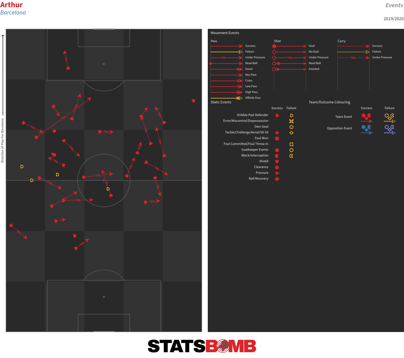 He’s also carried the ball further per 90 than any of the league’s other central midfielders.
 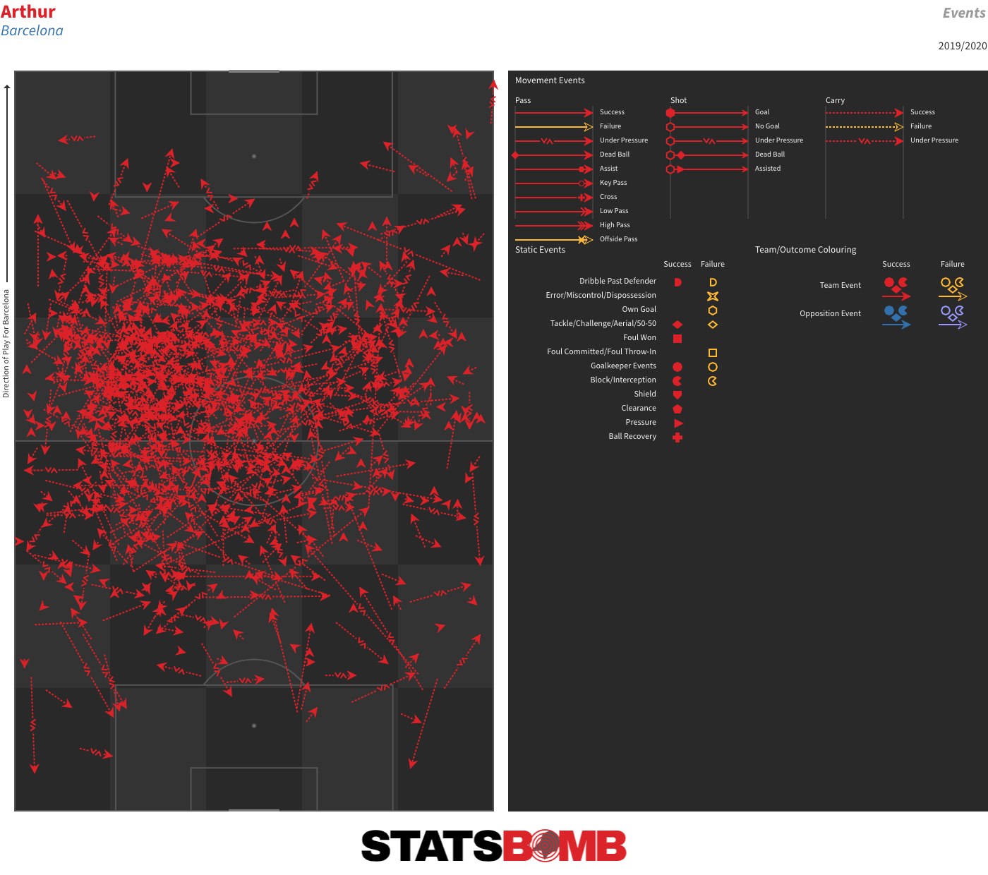 Add that to a very solid overall passing game and you have a player who probably deserved the benefit of at least another season to try and up his final-third output and offer a bit more defensively. Particularly so given how difficult it is to untangle some of his stagnant final-third output from the general attacking (and overall) decline at Barcelona. As it was, he represented the most sellable asset of a club who needed to balance their books. The fitness problems that have seen him miss a number of matches with knocks and niggling injuries arguably created enough doubts around him to justify Barcelona cashing in on him in a favourable deal. It’s just very hard to say that this was it.
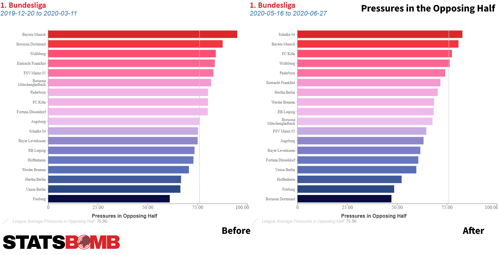
A historic Bundesliga season is in the books. As Germany’s top-flight managed to restart the season after the coronavirus-induced break sooner than the Premier League and La Liga, it experienced how the new environment affects the game earlier than others.
The Bundesliga staged nine matchdays under unusual precautions, most notably the banning of fans from the stadiums. It quickly became clear that--at least in this league--the home-field advantage was reduced when there weren’t tens of thousands cheering the team although this development has been overstated. In total, 37 out of 82 matches (81 matches on nine regular matchdays plus one match that was postponed before the break) were won by the away side, with nine of these wins for the underdog according to the standings. For comparison, we saw only 27 wins in the 80 matches on the nine matchdays before the break, including five underdog wins.
The empty stands undeniably affected the football played on the pitch. There’s a point to be made that football is less consequential when no one – besides the coaching staff and a handful of bench players – is reacting to success and failure. Especially early after the break, several Bundesliga players were keen to show that they can escape situations with elegance instead of brute force. This resulted in pressing attacks being outmanoeuvred with dribbles and smart movements while in normal times the long hoof might have been the typical reaction from defenders that don’t possess the best feet.
But that’s just anecdotal. Let’s look at some of the numbers that indicate the various effects of the different environment in what Germans call Geisterspiele (ghost games). We compare the nine matchdays after the break with the nine before, starting on 20 December 2019.
Less intensity
The eye test suggested early on that teams were less intense, particularly in advanced positions defending against the build-up of the opponents. The high press has been a prominent feature of Bundesliga football for several years. Centre-backs with bad feet often fell victim to this kind of style, while coaches of smaller clubs sometimes decided to abandon any kind of constructive build-up play for security concerns. While the pressures in the opposing half averaged around 77 per team per match before the break, it fell to 66 after it. This significant change certainly proves the eye test correct. What’s also striking is how many teams didn’t necessarily change their overall approach as the ranking among the Bundesliga clubs has remained largely the same, with two exceptions: Schalke, somewhat surprisingly, recorded the most pressures in the opposing half after the break which goes to show that the team did not give up in the midst of a crisis but rather were not able to capitalise on its intensity. Meanwhile, Borussia Dortmund dropped from second down to rock bottom which might give Lucien Favre’s critics some new fodder, as BVB were already third from last in this category before they lost to Mainz and Hoffenheim late in the season.
The number of counterpressures across the entire pitch also declined, falling from around 35 to 30 per team per match. Borussia Monchengladbach were outstanding in this category post-break, while Dortmund and Wolfsburg were less active immediately after turnovers.

There are a few factors that contribute to these numbers, most importantly the unparalleled circumstances during and shortly after the break. Teams were not able to train as hard as they would have liked to for a couple of weeks, because close contact between players was not allowed. Hertha’s Bruno Labbadia and a few other head coaches stated how they could not practise any kind of intense pressing or just intense actions in general which hindered plans to bring their teams into a state where they could replicate or improve the effectiveness of pressing.
Moreover, the overall fitness level was likely below par when the Bundesliga returned on 16 May, but the tracking data provided through the Bundesliga indicated that teams were only running less and made fewer sprints on the first matchday post-break, and as time moved on, the numbers quickly approached pre-Corona levels.
No tactical changes
An instinctive response to these stats could be that coaches just adjusted the tactical setup of their teams to pay tribute to the circumstances. They accepted that their teams could not play such a high or even midfield press throughout the entirety of the match and instead settle for a more cautious style with a deeper back line and a more compact structure that would rely less on defensive actions and instead defend space more effectively.
However, the defensive distance, meaning the average distance from a team’s own goal from which they make defensive actions, remained almost the same, with a per-team average of 43.9 metres before and 44.9 metres after the break. It wasn't the case that suddenly a good portion of the league was sitting deep, hoping to keep opponents away from the goal. We also didn’t see a wave of tactical changes, as most coaches stuck to what they did before the break in terms of basic formations and the structures in all game phases.
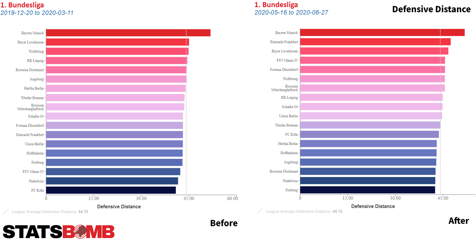
Higher xG
Less pressing coupled with no significant tactical changes could logically be considered to indicate a higher probability of scoring. Interestingly, on average, we saw fewer dribble attempts (17.3 compared to 18.3 per team per match) and fewer passes inside the box (2.4 compared to 2.7 before) but with a fairer distribution across the league. This indicates that it was easier for most of the teams to get close to the goal without having to rely on attacking actions that require outstanding individual skills. Instead, it was due to the declining resistance of opponents that teams were simply able to advance more easily.
The open play xG rose from an average of 1.06 to 1.13 per team per match. The average amount of shots per team per match, however, dropped from 13.12 to 12.32, with fewer shots resulting from a high press (3.0 to 2.5) and through counterattacks (1.3 to 1.1).
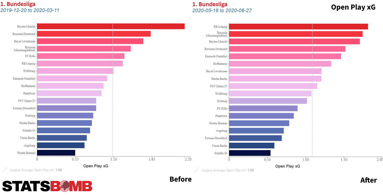
Overall, the attacking output did not increase, even though the decline in defensive intensity could have facilitated the output. What happened in the past few weeks was that there were fewer interactions between players, particularly in one-on-one duels, which allowed teams to play their way through defensive structures facing less resistance than usual. If the declining defensive resistance was caused from a lack of fans inspiring players to get physical, pressure opponents, and generate turnovers is just one factor in play during this period and is therefore up to debate, and a hypothesis that can perhaps never effectively be tested.
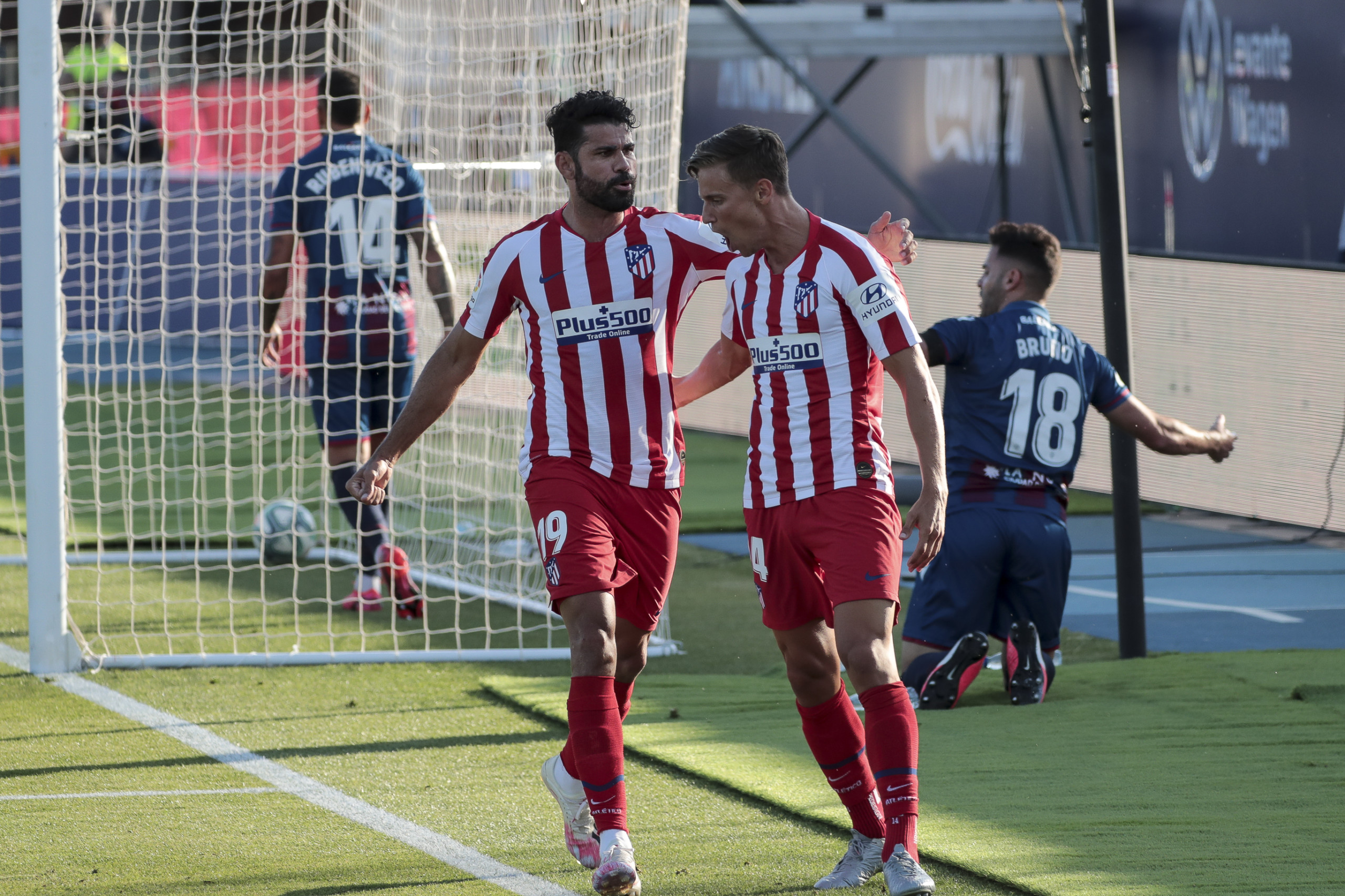
With a daily dose of partidos, writing about La Liga feels very much like shooting at a moving target right now, but we’ll do our best.
The New Reality
La Liga is back, and much looks the same as before. Valencia are still conceding shots at an alarmingly high rate, Messi continues to bear outsize responsibility for the success of the Barcelona attack, and André Zambo Anguissa remains one of the league’s most active dribblers and ball carriers through midfield.

There has been very little variation in the number of dribbles attempted and completed, in how quickly teams move forward and in how high up the pitch they defend. The ball has been in play for more or less the same amount of time. A comparable number of free-kicks have been conceded, and the overall number of pressures and counterpressures has remained more or less constant.
But some things have changed. We’re still dealing with a very low sample size here, so caution should be exercised in drawing any concrete conclusions, but a few patterns stand out.
La Liga was already the major European league that saw the least shots and expected goals (xG) per match, and those figures have fallen even further since the restart. The number of shots has dropped from a pre-stoppage average of 22.36 per match down to 19.91, while the average xG has gone down from 2.12 to 1.92. It seems teams have struggled to successfully advance into dangerous areas as often as before. Completed passes within 20 metres of the opposition goal are down by over 15%.
The aggressiveness with which teams are contesting possession has also decreased. On average, teams are allowing over one extra pass for each intent to break up opposition passing chains. The number of pressures in the attacking half and the proportion of aggressive actions (tackles, pressure events and fouls recorded within two seconds of an opposition ball receipt) are also down.
Llorente's New Role at Atlético
Atlético Madrid have been in fine form since the restart, recording three wins and a draw to take advantage of slower starts from other Champions League contenders and move up into third, six points clear of Getafe in fifth.
Diego Simeone’s side have had good underlying numbers all season, but a finishing slump that lasted all the way into early February meant that results didn’t follow. At that stage, they were running well over seven goals behind expectation, and all four of their primary forwards were underperforming their individual xG sums.
Things do now seem to be evening themselves out. Atlético have performed four and a half goals ahead of expectation over their subsequent nine matches, yielding an unbeaten run of five wins and four draws.
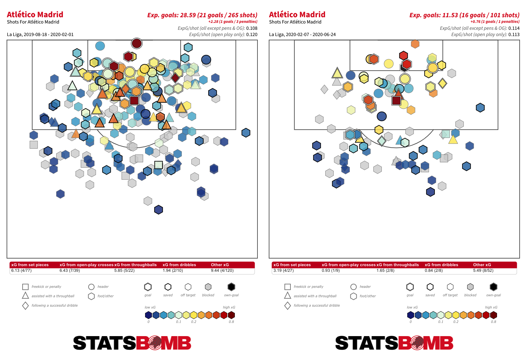
That surge primarily seems to be the result of a shift in fortune in front of goal, but Atlético’s results since the restart also have a fair bit to do with just how well Marcos Llorente has performed in an unfamiliar second striker role.
We got a glimpse of the possibilities in Atlético’s dramatic Champions League triumph over Liverpool just before the shutdown. There, Llorente was involved in all three of their extra-time goals, scoring twice and then slipping Álvaro Morata in behind for the third.
But few could have expected him to resume the campaign in an offensive role. A defensive midfielder by trade, there had been little in his performances at previous clubs or even at Atlético, where he hadn’t slotted in quite as well as expected, to suggest he had the skillset to thrive further up the pitch. His passing has always been more neat and tidy than incisive, and he’s never been even a medium-volume dribbler.
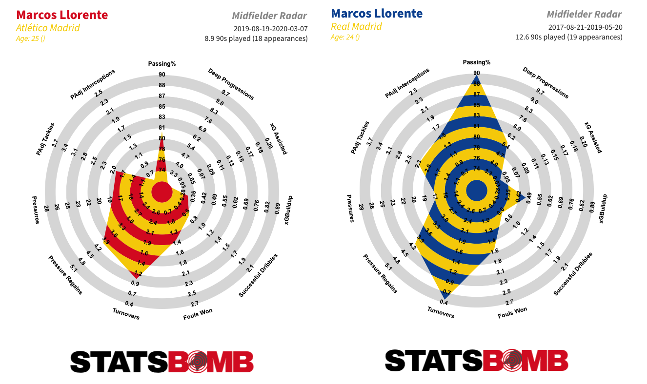
Simeone, though, had seen something. “After watching him in the training sessions, we decided to push him further forward against Liverpool and we discovered a player with different characteristics to the others in that position,” he explained after Llorente provided his third assist since the restart in Atlético’s 1-0 win away to Levante on Tuesday. A repeat of the surprisingly deft footwork that led to his goal against Osasuna this time produced space for a cutback deflected into his own net by Bruno González.
In just 231 minutes of football, Llorente has already completed double the number of dribbles he did in the previous 812...
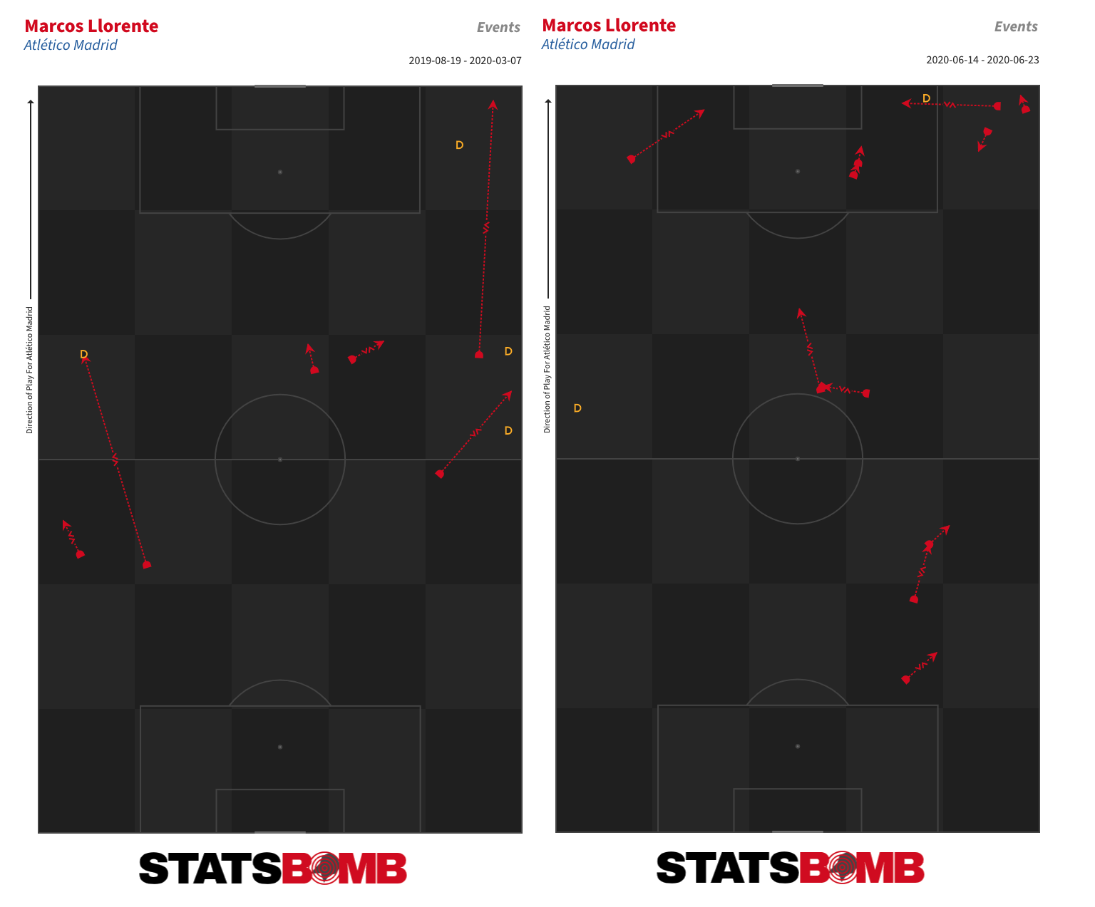
...and has set up more chances than the previous season and a half combined. After two seasons without completing a through ball, he has slipped through two in a week and a half. We are working with a super small sample size here, and it remains to see how much of this will hold over a larger one, but it appears that Simeone might just have engineered himself a new forward.
Betis Sack Rubi
It had been coming for a while, and finally the axe fell. Real Betis parted ways with head coach Rubi on Sunday following a 1-0 defeat away to Athletic Club that left them without a win since the restart and with just one in their last 10 matches.
Rubi produced an excellent seventh place finish at Espanyol last season but was unable to replicate the neat and progressive football of that side with what was, on paper at least, a more talented squad at Betis. The underlying numbers were okay -- upper, rather than lower, middle pack -- but not enough to offer stringent support for his continuation given the club’s budget and pre-season pretensions.
Rubi was never able to get on top of the defensive issues that led to his team conceding more goals than all but Espanyol and Mallorca, both of them relegation candidates. He also failed to derive any sort of output from summer arrival Borja Iglesias, signed for €28 million after an impressive season alongside Rubi at Espanyol. This is just pitiful:
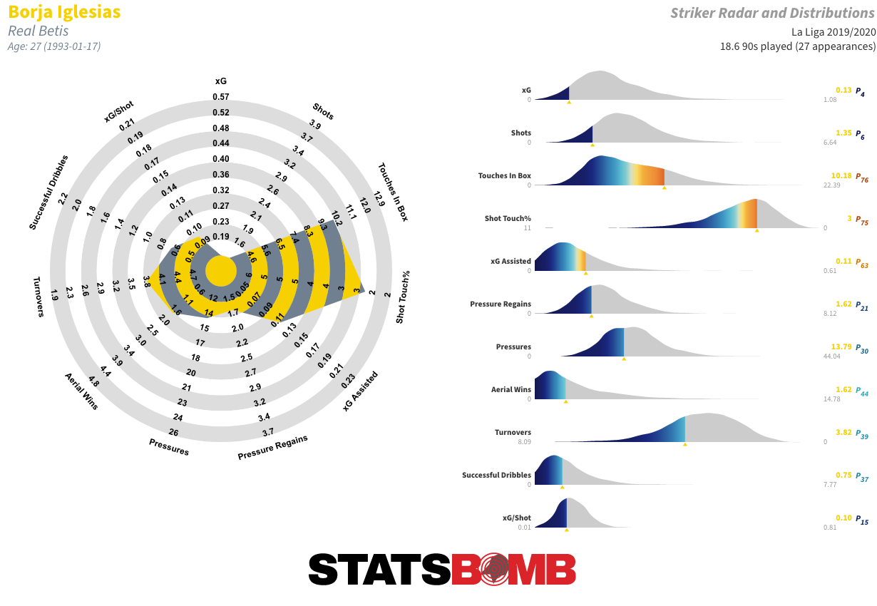
The reintroduction of elements of the approach of his predecessor Quique Setién did power a promising run of results through the back end of 2019 into the new year that was backed up by strong underlying numbers. But that swiftly petered out as attacking output cratered and their defensive numbers began to waver. Over the course of Rubi’s final 10 matches in charge, Betis were back to a pretty much even xG difference. More damagingly, they took just seven points -- alongside Eibar, the joint-lowest mark in the league.
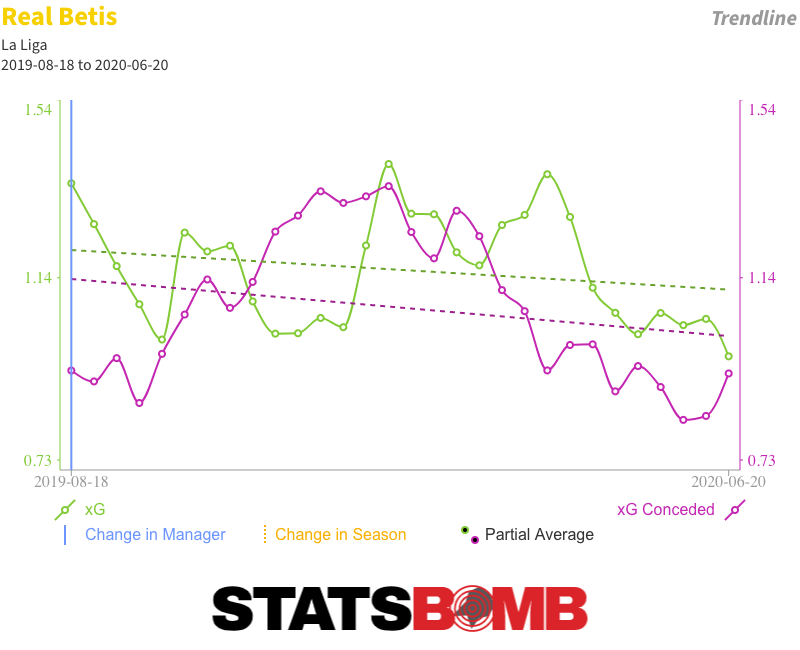
Rubi leaves Betis down in 14th, clear of the bottom three but with no realistic chance of European qualification. Another reset is in order. It seems that however much the directorship talk of modernising the club, this remains Betis: four head coaches and various backstage reshuffles in four seasons is about par de course at the Benito Villamarín. Alexis Trujillo takes charge until the end of the season, but who comes next? Javi Gracia, Manuel Pellegrini, maybe even Unai Emery?
La Liga is back. Nearly a month after the Bundesliga became the first of the major European leagues to resume, the Spanish top flight returns with an enticing set of fixtures that begin with a city derby between Sevilla and Real Betis on Thursday evening. Up and down the league, there is still much to be decided across the remaining 11 rounds of action. The Title Race Realistically, Barcelona and Real Madrid are the only two teams in the title race. Barcelona lead the way, two points clear of Madrid and a further nine ahead of Sevilla in third. The momentum would appear to be with the leaders. Since Quique Setién replaced Ernesto Valverde in January, they’ve taken more points than any other side in La Liga. Over that fairly small sample size of eight matches, they’ve also had the best expected goal difference, and by some distance: 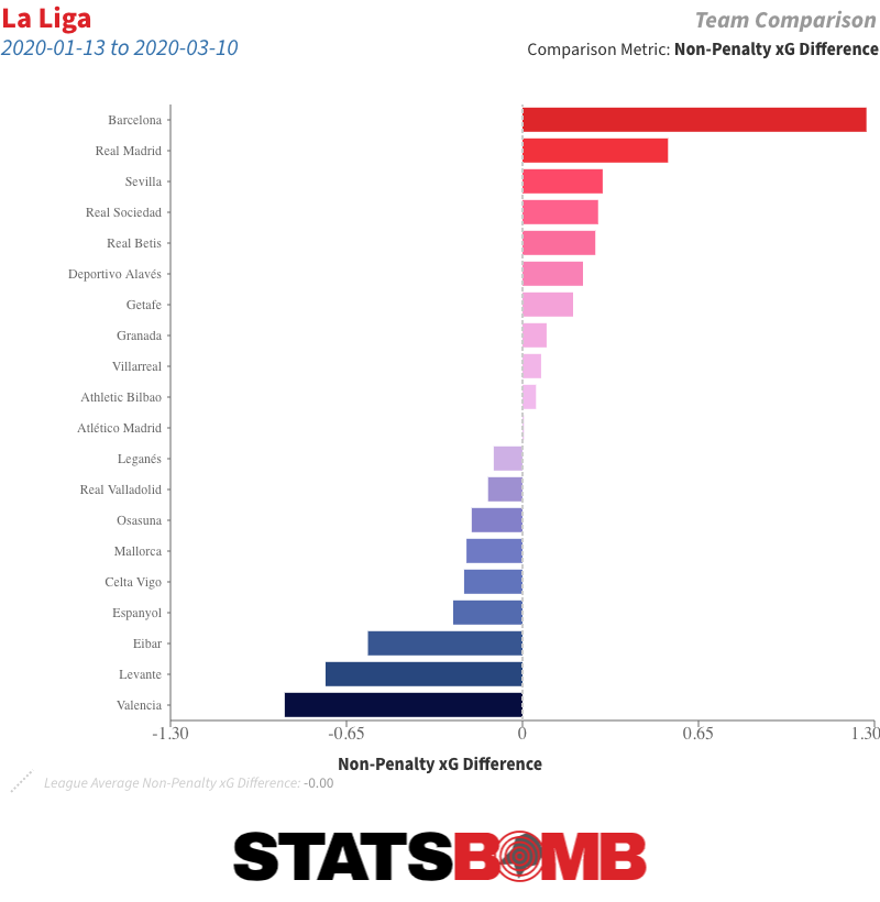 Setién’s heavily possession-based style should also be a good fit for the hectic fixture list that, if everything runs smoothly, will see the teams play their remaining 11 matches over the course of just over five weeks of action. There are some counterpoints. On paper, Madrid look to have the easier run-in. The pause has also given Eden Hazard the opportunity to recover from what seemed likely to be a season-ending injury. With Marco Asensio likewise closing in on a return, Madrid look better equipped than they might otherwise have been to go toe-to-toe for the title. European Places The contest for the two remaining Champions League places will be a thrilling watch. Just two points currently span Sevilla in third, Real Sociedad in fourth, Getafe in fifth and Atlético Madrid in sixth. Sevilla possibly have a slight edge. January signings Youssef En-Nesyri and Suso have added some needed variety to their attack, and while both Getafe and Real Sociedad have gained ground on them since the turn of the year, Sevilla’s underlying numbers have remained strong.
 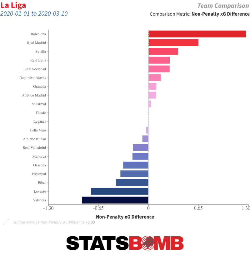 But this is a very difficult race to call. Real Sociedad have won admirers as a young and vibrant team playing attractive football, but they look to have the toughest schedule of any of the top-four aspirants. Getafe have been on a tear since the turn of the year, but can they maintain their intense play style through the crammed fixture list? With their finishing slump seemingly behind them, and with a fairly accessible run-in, can Atlético barge into the top four? What seems clearer is that the race is limited to those four teams. Valencia are only actually three points back from Atlético but seem to have had more than their fair share of fortune. They’ve consistently over-performed their poor underlying numbers.
 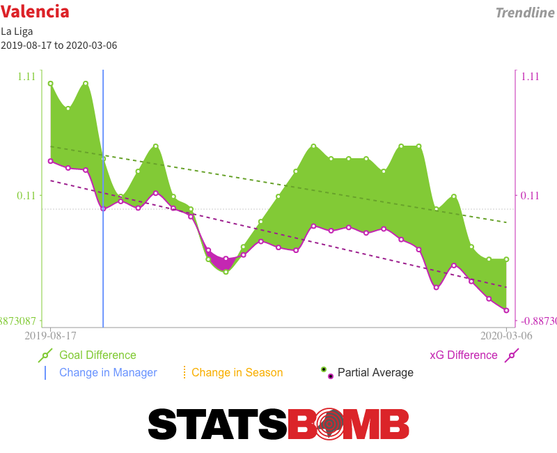 Valencia’s numbers are trending in the wrong direction, and it seems improbable that a team taking less than nine shots a match while conceding nearly 15 can continue to get the results necessary to keep pace with those ahead. In fact, their seventh place, a position that could yield a Europa League spot depending on the outcomes of domestic and continental cup competitions, could come under threat from behind. Villarreal have been frustratingly inconsistent but have enough quality in attack to make up the four-point difference if things go their way. Granada have impressed on their return to the top flight and made a good start to 2020. But that’s probably it. Athletic Club have one of the best defensive records in the league but their attacking output is below average, and they’ve benefited from a positive swing versus their underlying numbers. They’ve also taken just 11 points from their last 12 fixtures. The Copa del Rey final against Basque rivals Real Sociedad would seem to offer their best hope of European qualification. Relegation There are three relegation places to be filled and six teams trying to avoid them. While there is still an outside chance that Alavés or Levante might get dragged into it, the battle against the drop is likely to be contested by Espanyol, Leganés, Mallorca, Celta Vigo, Eibar and Real Valladolid. Espanyol are bottom of the pile. Results have improved considerably since Abelardo became their third head coach of the campaign late into December, but there hasn’t been an accompanying improvement in their underlying numbers. In that time, they’ve been one of the league’s worst sides:
  With other teams towards the foot of the table also picking up good points in the lead up to the league stoppage, they are still six points shy of safety. All is not lost. There is still over a quarter of the campaign to be played. But Espanyol are not in a good position right now. Second from bottom are Leganés. They’ve had mid-table underlying numbers all season but have consistently underperformed those numbers at both ends of the pitch.
  Their luck may yet turn, but the January departures of En-Nesyri and Martin Braithwaite, between them scorers of almost half of their league-low tally of 21 goals, certainly didn’t help their cause. Next up are Mallorca, Celta Vigo and Eibar, all separated by just two points between 18th and 16th. Mallorca have shown signs of improvement since the turn of the year, particularly in defence, but they have one of the hardest closing schedules and a thin squad. Things look brighter for Celta Vigo, who have been a lot better under Óscar García and added players in three key positions during the January window.
 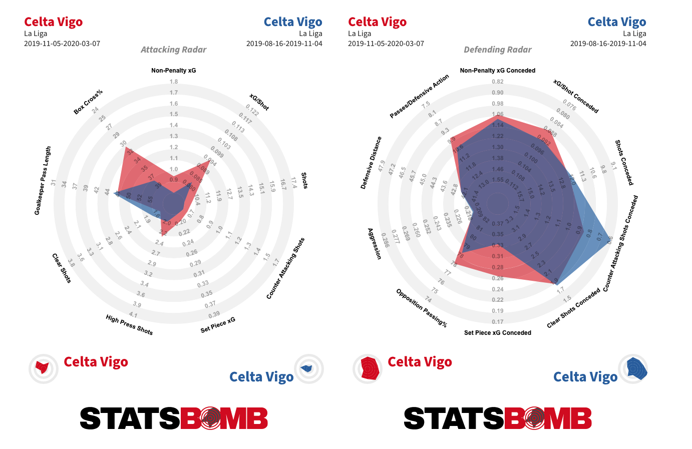 Eibar might be in trouble. While they’ve improved upon their pitiful early season performances, they’ve still been one of the worst three teams in the division by the underlying numbers since the turn of the year. A combination of the league’s oldest squad and an aggressive play style is unlikely to mesh well with the condensed schedule. Valladolid have a four-point cushion over the last relegation place. While they are far from home and dry, if they can continue to pick up points at their current rate -- which seems doable considering they are performing pretty much exactly in line with their underlying numbers -- it is unlikely that three teams will overtake them.
We complete our data history of the European Cup with the all-Bundesliga final of 2013. After seeing off the Spanish giants in their semi-finals, Bayern Munich and Borussia Dortmund met at Wembley, each seeking to become the first German winner in over a decade. This is the sixth and final part of the series.
We’ve previously covered: - 1960: Real Madrid 7 - 3 Eintracht Frankfurt - 1972: Ajax 2 - 0 Inter Milan - 1989: AC Milan 4 - 0 Steaua Bucharest - 1995: Ajax 1 - 0 AC Milan - 2009: Barcelona 2 - 0 Manchester United
Bayern were the favourites coming into the match, having run away with the Bundesliga and traversed a difficult route to the final that included a historic 7-0 aggregate thrashing of Barcelona in the final four; Dortmund had come ever so close to elimination against Málaga in the last eight before then seeing off Real Madrid to make it through to the final.
Bayern had been extremely unfortunate to lose out to Chelsea in the 2012 final and were seeking to make amends and send coach Jupp Heynckes off into retirement on a high with victory.
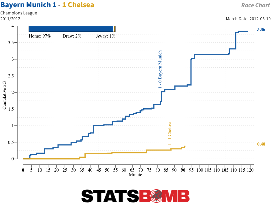
New Style, Vintage Results
Just as we seemed to have settled into a stylistic tussle between patient possession and deep block defending, along came the Germans to upset the apfelkarren. Suddenly, the attention of the footballing world shifted to the Bundesliga. Gegenpressing (later translated as counterpressing) firmly entered the football lexicon and there was much talk of the importance of transitional phases of play.
The meeting of two German sides at Wembley produced a high-paced encounter that was actually closer in style and output to the 1960 final that any of the others we’ve covered in this series. The shot count was nowhere near as high, but the 2013 final nevertheless sits second only to 1960 in terms of the expected goals (xG) total, although that was heavily tilted towards Bayern.
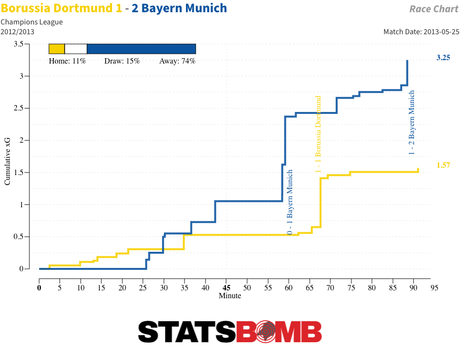
There was also some of the frantic, back-and-forth play of that early final on display. The average speed of attack was the fastest of all the finals we’ve covered, faster still than in 1960. Dortmund were especially swift to transition forward after gaining possession.
The average pace towards goal for teams in last year’s Champions League was 2.53 metres per second; Dortmund raced forward at a rate of 4.61 metres per second. Not that it lead to a particularly dangerous set of shots. Jurgen Klopp’s team began on the front foot, getting off six efforts on goal before Bayern had even mustered one, and accumulated 12 over the course of the 90 minutes.
But even with Robert Lewandowski, scorer of all four goals in Dortmund’s 4-1 thrashing of Real Madrid in the first leg of their semi-final and impeccable in his use of his body to shield the ball and turn defenders, and an effervescent Marco Reus among their starts, they not only managed five less shots than Bayern, but the average quality of those shots was also far below those of their opponents. Despite a heavily aerial attack, there was very little fat on the Bayern shot map.
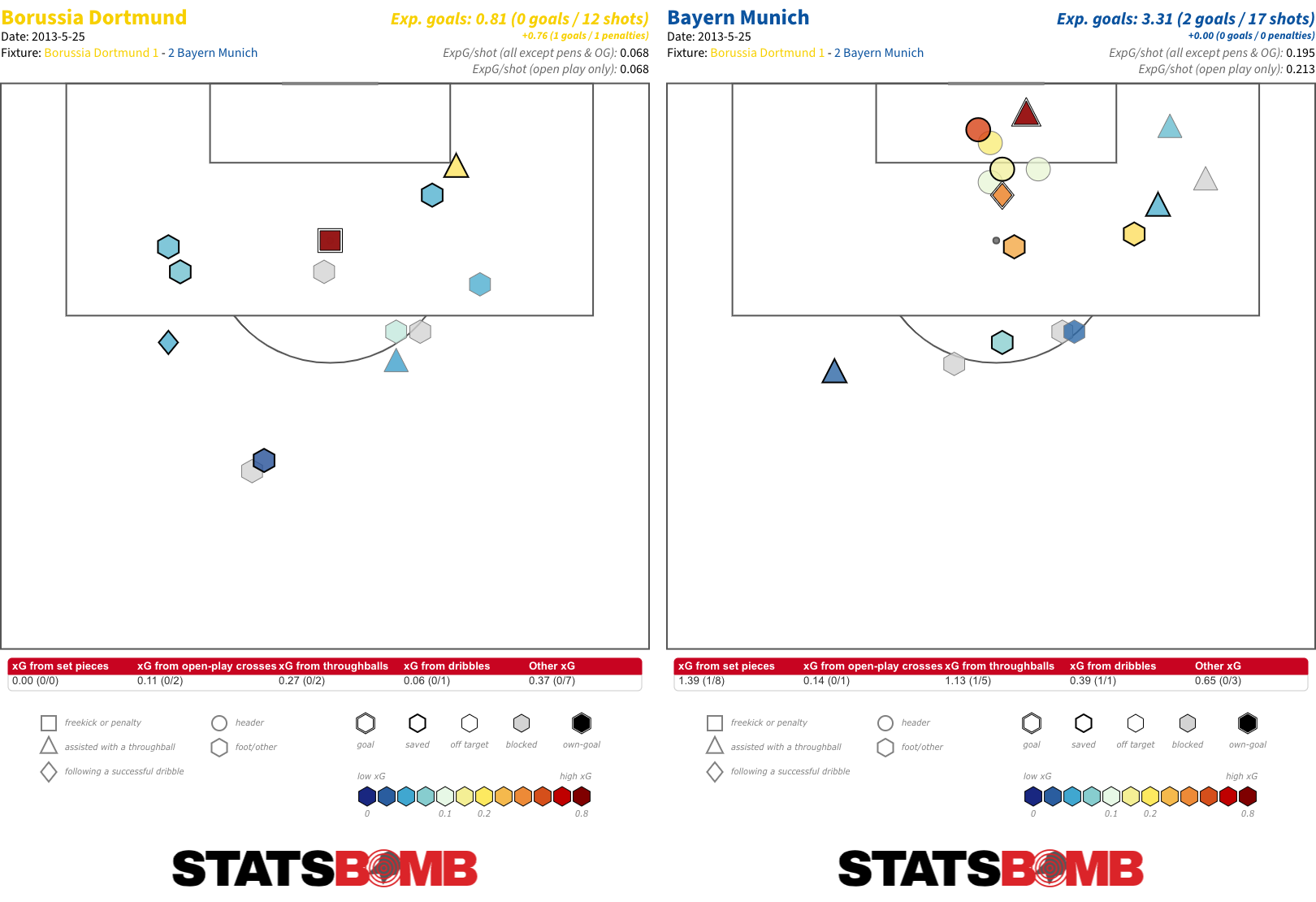
Remove Dortmund’s penalty from the equation and they created under one expected goal. It may have taken Bayern until the 89th minute, when Arjen Robben skipped between two defenders and finished neatly to finally enjoy success in a major continental final after two failed attempts at the Champions League with Bayern and a World Cup final defeat with the Netherlands, to score their winner but it was clearly deserved. Robben and Thomas Müller had been involved in much of their best play.
The pace with which the two teams attacked saw them regularly turn over possession. Even Bayern’s more patient buildup in deeper areas usually eventually resulted in a long ball forward from one of the two central defenders.
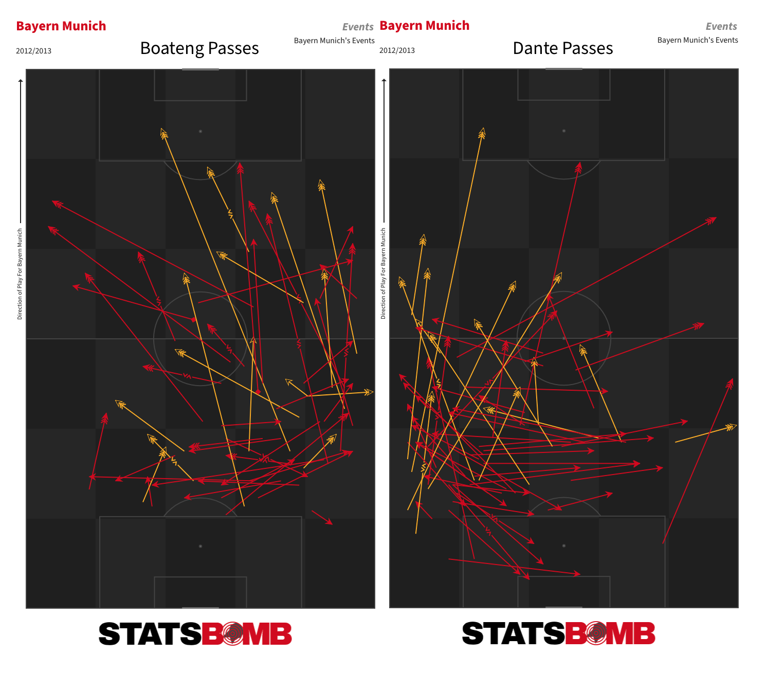
The final featured the lowest passing completion percentage of any since 1960, with just a 71% completion rate -- nearly four percentage points fewer than the next lowest. Dortmund’s 65% rate was the first time since 1960 that a team had dipped below 70%.
Not only did it stand out in comparison to the other finals in this series but also within the context of contemporary finals. The completion rate was the lowest of all those contested in the 2010s. [table id=82 /] And that’s the thing. For all that this was heralded as a new dawn in football, it didn’t start a revolution nor did it herald a new era of German dominance.
The national team won the following year’s World Cup, but did so with a more possession-dependent style of play. At club level, Spain came back strongly, with Barcelona and Real Madrid lifting the Champions League trophy in each of the subsequent five seasons -- four times in Madrid’s case.
Germany is yet to provide another finalist.
Such is the widespread availability of footage in the modern age that even before Bayern and Dortmund took to the pitch at Wembley, their ideas had already been acutely analysed and elements incorporated elsewhere.
They didn’t enjoy the same sort of extended advantage that a novel play style afforded Inter Milan in the 1960s or Ajax in the 1970s, for example. The totals for counterpressures and counterpressures in the respective attacking thirds in this match fell on or below the average points for those metrics during last season’s Champions League.
What was once unique quickly became commonplace.
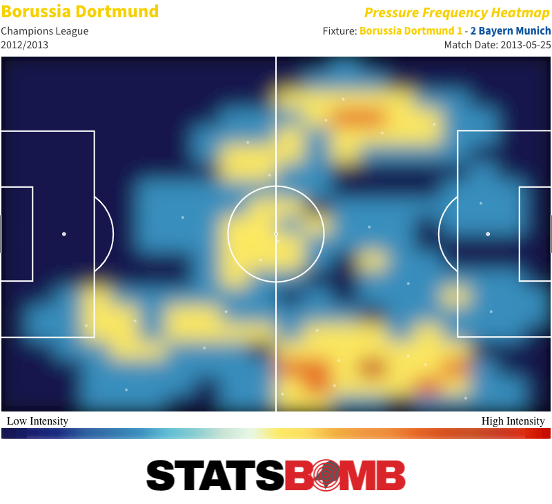
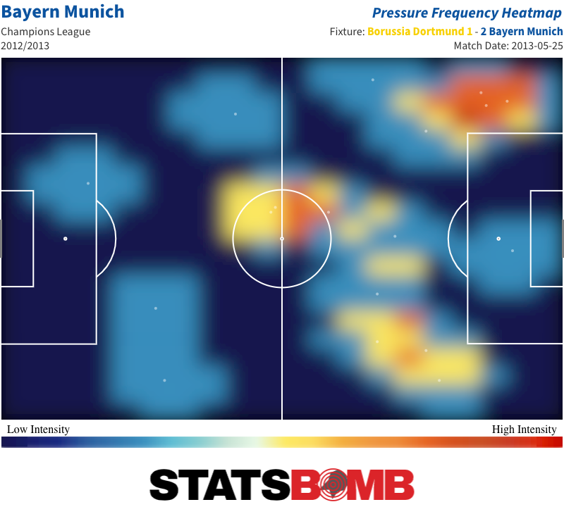
Pep Guardiola’s arrival at Bayern in the summer of 2013 and some of his innovations, including narrowly positioned full-backs, also provided ready examples of how possession-based teams might seek to better protect themselves against rapid transitions. Add all that up and this final almost feels like a rapidly resolved glitch in the system.
Dangerous Bayern Corners
This Bayern side were a real force from set-pieces. Two of the goals in their semi-final rout of Barcelona had come from them, and they also created numerous chances from corners in the final. Seven shots from eight corners and pretty much an entire expected goal.
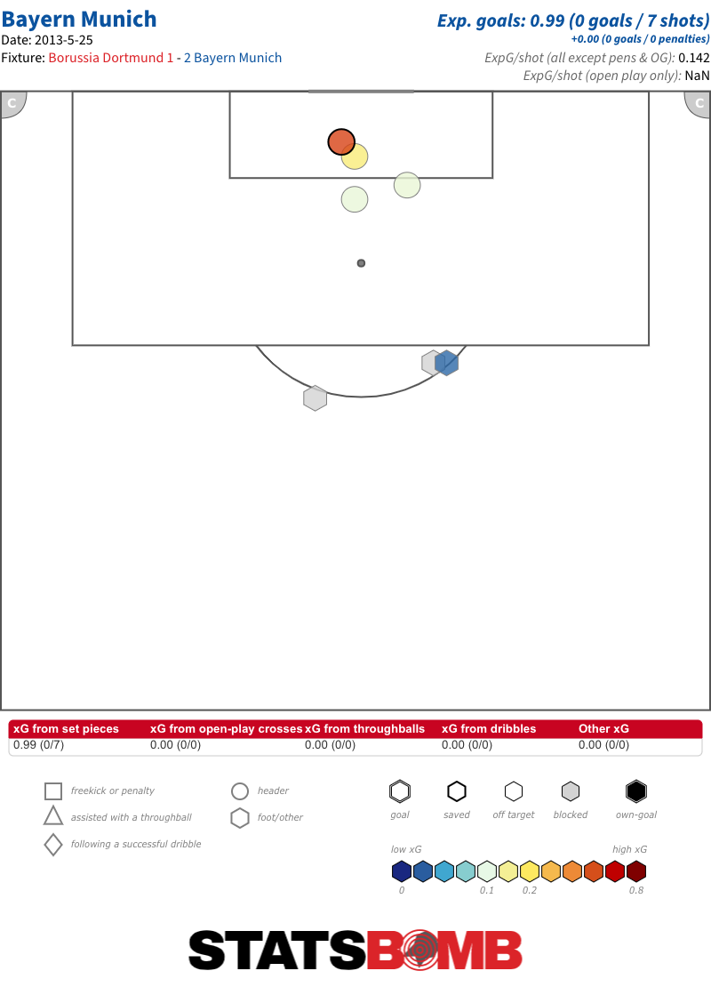
There wasn’t all that much sign of some of the more advanced routines we see these days, although a neat early free-kick scheme saw Thomas Müller drop off to receive a central pass and lay wide for a cross headed on goal by Mario Mandzukic.
The same player was unable to adjust his body sufficiently to successfully convert a near-post flick from a right-wing corner. But in Mandzukic, Müller and Javi Martínez, Bayern had three players very much capable of winning individual duels to get on the end of deliveries.
------------------------------
We hope you’ve enjoyed this series. Alongside our release of the Arsenal Invincibles data earlier this week, we also made our data from each of the last 20 Champions League finals freely available. If you fancy digging into some of the competition’s recent history, all the details for accessing the data can be found here.
And a complete primer (in English and Espanol) on how to work with the data via StatsBombR is here.
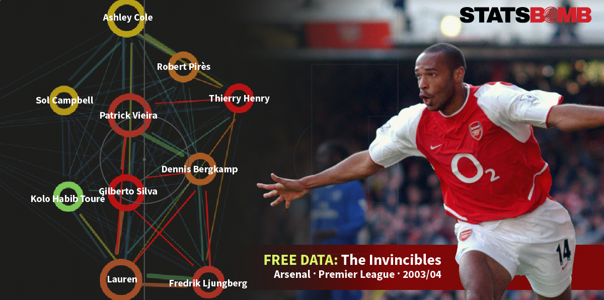
As those of you who follow me on social media are aware, earlier this year we started working on The Invincibles Project. The idea behind this was to collect all of the data from this historic season to be able to look at it through a modern lens. I had initially pitched this as a follow-up project after the Messi Data Biography as something different, and another way of unlocking football's history.
As an Arsenal fan, I found the whole thing exciting. Prime Thierry Henry! Doing things like this:
The majesty of Robert Pires. Taking bodies!
Dennis Bergkamp! Patrick Vieira! Jose Antonio Reyes! Kolo kolo Toure! Sol Campbell! Mad Jens!
*Highbury roars*
OMG SO EXCITING.
Cashley.
*crickets chirping*
Also as an Arsenal fan, I know that other Arsenal fans could use a little joy in their lives and this seemed like the only way we were getting anything fun out of the Gunners in 2019-20.
We started collecting this with an eye to releasing it side by side with the data set from a different red team, should they manage to finish their season undefeated. Sorry Liverpool fans, due to circumstances beyond our control, that data release slipped through our fingers. You'll have to settle for merely a league title and one of the largest title winning margins in history.
The Problem
In order to collect data, we need to have video. It was fortunate for us that Lionel Messi has played his entire career for Barcelona, because that is one of the few teams in the world that has historic video available on the internet from pre-2010 without needing to jump through a million hoops. That doesn't mean that getting all of the video to reconstruct Messi's club career was easy - far from it. It was merely doable.
Arsenal? The only undefeated season in Premier League history? You would think this would be at least as simple as sourcing 15 seasons of Messi, right?
It was not.
We managed to get about half the 2003-04 season from the usual sources of football video history. And then we hit a wall. Our man in Spain and historic video expert Pablo Rodriguez then went to work, checking with various and sundry collectors that he knows who have large archives of historic, important football video. Through these wonderful people and the standard exchange of goods and services we were able to get to 32 matches of video. And then we hit another wall.
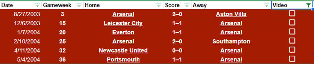
Why? well as Andrew Mangan of Arseblog reminded me, not all matches during that time period were broadcast to TV. In the modern day, every Premier League match is broadcast to air in multiple countries, which makes it easy to grab that video and store it away on a giant hard drive. Back then? A number of 3PM matches on Saturdays were simply never broadcast. (At least to our knowledge.) Which means that the collectors would not have that video unless they somehow tapped into different sources.
We checked with Arsenal. I've been lucky enough to meet people that work for the club over the years, and we figured maybe they would let us have access to the video to collaborate on the data release and some cool stuff with club media. And they totally would have been...
Except they didn't have the video either.
Someone who worked for Prozone back in the day suggested that the opponents might have those videos, as they would have been delivered by courier as part of their service. But that ran into a variety of snags, including the fact that football clubs change personnel on this end with remarkable regularity, and having the archive, being able to access it, and even knowing who to talk to was insurmountable for us.
The other problem here is the transition from analog to digital. Pretty much all archives back then were tape archives that would later need to be digitised so the match would be preserved for history. Rob Bateman of Opta tells the tale of trying to collect old Premier League matches from the 90s and being surrounded by crumbling video tape from the league's first decade. These Arsenal matches came right at the tail end of that period, and my understanding is that the PL has started to archive its history as much as possible, but it's still very much a work in progress.
Finally you hit the problem of a license fee. We got in touch with the archive service with a willingness to pay a fee to obtain the final six matches needed to complete the project. We were quoted a figure to license the video for the entire Arsenal season that frankly didn't make any sense to me, and certainly eclipsed my budget for a public service project.
I wanted to get everyone a data gift to bring people some joy during the pandemic, but I didn't want to/could not pay the price of a car to make that happen.
The Premier League itself actually showed willingness to help us out, but as you can understand, they are rather busy with other priorities right now (like restarting the league during the middle of a viral pandemic) and suggested maybe we can revisit this when the world wasn't quite so mad? Which totally makes sense.
But I have an anniversary data release deadline, and thus here we are.
Incomplete Invincibles.
Classics Data Pack 1
To make up for my own disappointment in not being able to complete this project, I added some extra matches I thought might interest people, including non-Arsenal fans. So what you are getting today as a gift from Hudl Statsbomb is a hefty little slice of football history, wrapped in the above-named package. In addition to delivering 32 of 38 matches from the Arsenal 2003-04 Premier League season, we are also giving you UEFA Champions League Finals data from 2000-2019. The collection on those CL matches aren't all finished, so will trickle out to the repository gradually over the next week to complete the set.
Thank you to all of the fans out there who have supported Hudl Statsbomb over the years. Thank you to our customers who buy our products and give us feedback to make us better every day.
And thanks to Arsenal for a truly magnificent season and set of memories. It would be great if we could get some more of those sooner rather than later. Information on how to access the data is here
A complete primer (in English and Espanol) on how to work with the data via Hudl StatsbombR is here
*EDIT: A new, updated version of the R Guide can be found here
The data comes with our standard non-commercial license that is usable for fan analysis and academic research. If you are a commercial entity that would like to use this data, get in touch with sales@statsbomb.com and we can have a conversation.
All the best,
--Ted Knutson
CEO, StatsBomb
*If we get video and I still run StatsBomb, we will finish this project.